Ultimate guide to optimizing Stable Diffusion XL
Discover how to get the best quality and performance in SDXL with any graphics card.
Introduction
In this article we're going to optimize Stable Diffusion XL, both to use the least amount of memory possible and to obtain maximum performance and generate images faster. We will be able to generate images with SDXL using only 4 GB of memory, so it will be possible to use a low-end graphics card.
We're going to use the diffusers library from Hugging Face since this blog is scripting/development oriented. Even so, learning the different optimization techniques and how they interact with each other will help us take advantage of them in all types of applications, such as Automatic1111's Stable Diffusion web UI or, especially, ComfyUI.
The article may seem long and dense, but you don't have to read it all at once. My goal is to make you aware of the different optimization techniques that exist and to teach you when and how to use and combine them, although some of them already make a substantial difference on their own.
You can jump directly to the conclusions where you will find a table summarizing all the tests, as well as suggestions for when you're looking for quality, speed or ability to run the inference process with memory limitations.
Methodology
For testing I used the RunPod platform, generating a GPU Pod on Secure Cloud with a RTX 3090 graphics card. Although Secure Cloud is a bit more expensive than Community Cloud ($0.44/hr vs $0.29/hr), it seemed more appropriate for testing.
This instance was generated in the EU-CZ-1 region with 24 GB of VRAM (GPU), 32 vCPU (AMD EPYC 7H12) and 125 GB of RAM (CPU and RAM values don't matter much). As for the template I used RunPod Pytorch 2.1 (runpod/pytorch:2.1.0-py3.10-cuda11.8.0-devel-ubuntu22.04), a template that has the basics and nothing else. We don't care about the PyTorch version because we're going to change it, but this template offers Ubuntu, Python 3.10 and CUDA 11.8 as standard. In just 2 clicks and 30 seconds we already have everything we need.
If you're going to run the model locally, just make sure you have Python 3.10 and CUDA or equivalent platform installed (in this article we will use CUDA).
All tests have been performed within a virtual environment:
python -m venv .venv# Unix
source .venv/bin/activate
# Windows
.venv\Scripts\activateInstalling the following libraries:
pip install torch torchvision --index-url https://download.pytorch.org/whl/cu118
pip install transformers accelerate diffusers
The tests consist of generating 4 images and comparing different optimization techniques, some of which I'm pretty sure you haven't seen before. These differently themed images are generated with the stabilityai/stable-diffusion-xl-base-1.0 model, using only a positive prompt and a fixed seed. The rest of the parameters will be kept by default: empty negative prompt, size of 1024x1024, CFG value of 5 and 50 steps (sampling steps).
- Python
queue = []

# Photorealistic portrait (Portrait)
queue.extend([{
  'prompt': '3/4 shot, candid photograph of a beautiful 30 year old redhead woman with messy dark hair, peacefully sleeping in her bed, night, dark, light from window, dark shadows, masterpiece, uhd, moody',
  'seed': 877866765,
}])

# Creative interior image (Interior)
queue.extend([{
  'prompt': 'futuristic living room with big windows, brown sofas, coffee table, plants, cyberpunk city, concept art, earthy colors',
  'seed': 5567822456,
}])

# Macro photography (Macro)
queue.extend([{
  'prompt': 'macro shot of a bee collecting nectar from lavender flowers',
  'seed': 2257899453,
}])

# Rendered 3D image (3D)
queue.extend([{
  'prompt': '3d rendered isometric fiji island beach, 3d tile, polygon, cartoony, mobile game',
  'seed': 987867834,
}])
These are the images that are generated by default:


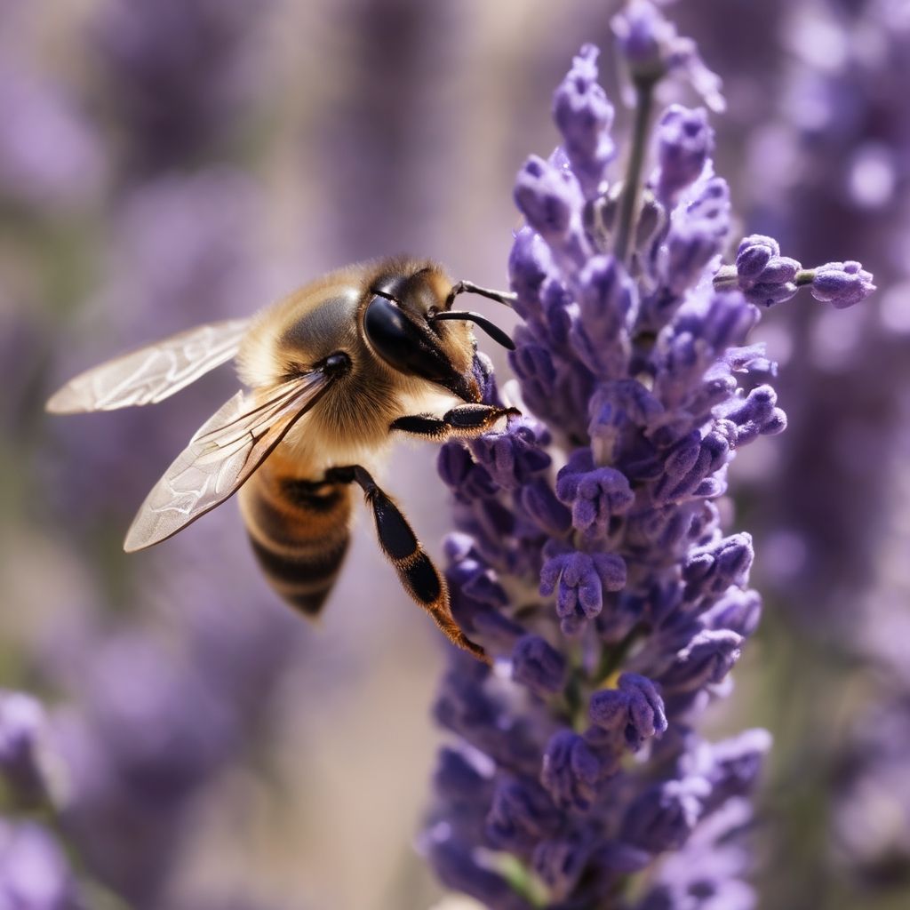

The following results are compared:
- Perceived quality of the images (I hope to be a good judge).
- Time it takes to generate each image, as well as total compilation time if any.
- Maximum amount of memory that has been used.
Each test has been run 5 times and the average value was used for comparisons.
Time measurements have been made using the following structure:
- Python
from time import perf_counter
# Import libraries
# import ...

# Define prompts
# queue = []
# queue.extend ...

for i, generation in enumerate(queue, start=1):
  # We start the counter
  image_start = perf_counter()

  # Generate and save image
  # ...

  # We stop the counter and save the result
  generation['total_time'] = perf_counter() - image_start

# Print the generation time of each image
images_totals = ', '.join(map(lambda generation: str(round(generation['total_time'], 1)), queue))
print('Image time:', images_totals)

# Print the average time
images_average = round(sum(generation['total_time'] for generation in queue) / len(queue), 1)
print('Average image time:', images_average)
To fint out the maximum amount of memory that has been used, the following line is included at the end of the file:
- Python
max_memory = round(torch.cuda.max_memory_allocated(device='cuda') / 1000000000, 2)
print('Max. memory used:', max_memory, 'GB')
What you will find in each test will be the minimum code required. Although each test has its own structure, the code is more or less like this:
- Python
# Load the model on the graphics card
pipe = AutoPipelineForText2Image.from_pretrained(
  'stabilityai/stable-diffusion-xl-base-1.0',
  use_safetensors=True,
  torch_dtype=torch.float16,
  variant='fp16',
).to('cuda')

# Create a generator
generator = torch.Generator(device='cuda')

# Start a loop to process prompts one by one
for i, generation in enumerate(queue, start=1):
  # Assign the seed to the generator
  generator.manual_seed(generation['seed'])

  # Create the image
  image = pipe(
    prompt=generation['prompt'],
    generator=generator,
  ).images[0]

  # Save the image
image.save(f'image_{i}.png')To make the tests more realistic and less time-consuming, the FP16 optimization will be used in all tests.
Many of these tests are performed using pipelines from the diffusers library, in order to abstract complexity and have a cleaner and simpler code. When the test requires it, the abstraction level will be lowered, but ultimately we will always use methods provided by this library. Additionally, models are always loaded in safetensors format using the use_safetensors=True property.
The images you will see in the article are displayed with a maximum size of 512x512 for easy reading, but you can open the image in a new tab/window to view it in its original size.
You will find all the tests in individual files inside the blog repository on GitHub.
Let's get started!
Base optimizations
The basic and essential to start with, optimizations at library and model level.
CUDA and PyTorch versions
I started this test wondering if there would be a difference between using CUDA 11.8 or CUDA 12.1, as well as possible differences between the different versions of PyTorch, always above version 2.0.
| Inference time | Memory | |
|---|---|---|
| CUDA 12.1 + PyTorch 2.2.0 | 14.2s | 11.24 GB |
| CUDA 12.1 + PyTorch 2.1.2 | 14.2s | 11.24 GB |
| CUDA 11.8 + PyTorch 2.2.0 | 14.1s -0.7% | 11.24 GB |
| CUDA 11.8 + PyTorch 2.1.2 | 14.1s -0.7% | 11.24 GB |
| CUDA 11.8 + PyTorch 2.0.1 | 14.2s | 11.24 GB |
Well... what a disappointment, they all have the same performance. The differences are so small that perhaps they disappear if I do a larger number of tests.
Which one to use: I still have a theory. CUDA version 11.8 has been with us longer, so it makes sense that libraries and applications would perform better in this version than in a newer one. On the other hand, as for PyTorch, the more modern the version, the more functionality it should offer and the fewer bugs it should include. Therefore, even if it's placebo, I will stick with CUDA 11.8 + PyTorch 2.2.0.
Attention mechanisms
In the past, attention mechanisms had to be optimized by installing libraries such as xFormers or FlashAttention.
If you're wondering why these optimizations aren't mentioned in this article, it's because they're no longer needed. Since the release of PyTorch 2.0, the optimization of these algorithms is integrated into the library itself through various implementations (such as these two mentioned). PyTorch will use the appropriate implementation based on the inputs and the hardware in use.
FP16
By default Stable Diffusion XL uses the 32-bit floating point format (FP32) to represent the numbers with which it works and performs calculations.
The obvious question is... can the precision be lowered? The answer is yes. By using the parameter torch_dtype=torch.float16, the model is loaded into memory in half-precision floating point format (FP16). To avoid performing this conversion constantly we can download the model in FP16 format, since that variant is distributed. Simply include the variant='fp16' parameter.
- Python
pipe = AutoPipelineForText2Image.from_pretrained(
  'stabilityai/stable-diffusion-xl-base-1.0',
  use_safetensors=True,
  torch_dtype=torch.float16,
  variant='fp16',
).to('cuda')

generator = torch.Generator(device='cuda')

for i, generation in enumerate(queue, start=1):
  generator.manual_seed(generation['seed'])

  image = pipe(
    prompt=generation['prompt'],
    generator=generator,
  ).images[0]

  image.save(f'image_{i}.png')


| Inference time | Memory | |
|---|---|---|
| FP32 | 41.7s | 18.07 GB |
| FP16 | 14.1s -66.19% | 11.24 GB -37.8% |
By working with numbers that are half the size, memory usage drops dramatically and the speed at which calculations are performed increases considerably.
The only "negative" point is a loss of quality in the generated image, but it's practically impossible to see any difference because FP16 is still sufficient.
Furthermore, thanks to the variant='fp16' parameter we save disk space since this variant occupies half the size (5 GB instead of 10 GB).
When to use: Always.
TF32
TensorFloat-32 is a format halfway between FP32 and FP16, used in some NVIDIA graphics cards (such as the A100 or H100 models) to perform calculations using the tensor cores. It uses the same bits as FP32 to represent the exponent and the same bits as FP16 to represent the decimal part.
Although in our test bench (RTX 3090) calculations cannot be performed with this format, something curious happens that you surely won't expect.
Two properties are used to activate this numerical format: torch.backends.cudnn.allow_tf32 (which is activated by default) and torch.backends.cuda.matmul.allow_tf32 (which should be activated manually). The first enables TF32 in convolution operations performed by cuDNN and the second enables TF32 in matrix multiplication operations.
That the torch.backends.cudnn.allow_tf32 property is enabled by default regardless of your graphics card is a bit strange, isn't it? Let's see what happens if we disable this property by assigning it the value False.
- Python
torch.backends.cudnn.allow_tf32 = False
# it's already disabled by default
# torch.backends.cuda.matmul.allow_tf32 = False

pipe = AutoPipelineForText2Image.from_pretrained(
  'stabilityai/stable-diffusion-xl-base-1.0',
  use_safetensors=True,
  torch_dtype=torch.float16,
  variant='fp16',
).to('cuda')

generator = torch.Generator(device='cuda')

for i, generation in enumerate(queue, start=1):
  generator.manual_seed(generation['seed'])

  image = pipe(
    prompt=generation['prompt'],
    generator=generator,
  ).images[0]

  image.save(f'image_{i}.png')
Additionally, and out of curiosity, I've carried out tests using an NVIDIA A100 graphics card with TF32 enabled.
- Python
# it's already activated by default
# torch.backends.cudnn.allow_tf32 = True
torch.backends.cuda.matmul.allow_tf32 = True

pipe = AutoPipelineForText2Image.from_pretrained(
  'stabilityai/stable-diffusion-xl-base-1.0',
  use_safetensors=True,
).to('cuda')

generator = torch.Generator(device='cuda')

for i, generation in enumerate(queue, start=1):
  generator.manual_seed(generation['seed'])

  image = pipe(
    prompt=generation['prompt'],
    generator=generator,
  ).images[0]

image.save(f'image_{i}.png')To use TF32 you have to disable FP16, so we cannot use torch_dtype=torch.float16 nor variant='fp16'.
| Inference time | Memory | |
|---|---|---|
| Base | 14.1s | 11.24 GB |
| RTX 3090 - Disable TF32 | 14.2s +0.71% | 10.43 GB -7.21% |
| Inference time | Memory | |
|---|---|---|
| Base (FP32) | 34.4s | 18.07 GB |
| A100 - TF32 | 13.7s -60.17% | 18.07 GB |
| A100 - FP16 | 6.3s -81.69% | 11.24 GB -37.8% |
Using an RTX 3090, if we disable the torch.backends.cudnn.allow_tf32 property memory usage decreases by 7%. Why? I don't know, in principle I would say it's a bug since it makes no sense to enable TF32 on a graphics card that doesn't support it.
In the case of using an A100 graphics card, using FP16 we manage to reduce the inference time and memory usage very substantially. Memory usage can be further reduced by disabling torch.backends.cudnn.allow_tf32 just like on the RTX 3090. As for using TF32, being halfway between FP32 and FP16... it cannot beat FP16.
When to use: In the case of graphics cards that do not support TF32, it's clearly a good idea to disable the property that is enabled by default. Using an A100 it's not worth using TF32 if we can use FP16.
Pipeline optimizations
These optimizations modify the pipeline to improve some aspects.
The first three modify when the different components of Stable Diffusion are loaded into memory so that they're not all loaded at the same time. These techniques achieve a reduction in memory usage.
Use these optimizations when necessary due to graphics card and memory limitations. If you get the error RuntimeError: CUDA out of memory on Linux, this is your section. On Windows there is virtual memory (Shared GPU memory) by default, and although its more difficult to receive this error, the inference time will increase exponentially, so this is also your section.
As for the last three optimizations in this section, they consist of libraries that optimize the pipeline in different ways to reduce inference time as much as possible.
Model CPU Offload
This optimization comes from the accelerate library. When a pipeline is executed all models are loaded into memory. With this optimization we tell the pipeline to move into memory only the model that is needed at each moment. This order can be found in the source code of the pipeline, in the case of Stable Diffusion XL we will find the following line:
- Python
model_cpu_offload_seq = "text_encoder->text_encoder_2->image_encoder->unet->vae"The code to implement Model CPU Offload is quite simple:
- Python
pipe = AutoPipelineForText2Image.from_pretrained(
  'stabilityai/stable-diffusion-xl-base-1.0',
  use_safetensors=True,
  torch_dtype=torch.float16,
  variant='fp16',
)

pipe.enable_model_cpu_offload()

generator = torch.Generator(device='cuda')

for i, generation in enumerate(queue, start=1):
  generator.manual_seed(generation['seed'])

  image = pipe(
    prompt=generation['prompt'],
    generator=generator,
  ).images[0]

image.save(f'image_{i}.png')Thanks to Terrence Goh who reminded me through Ko-fi that we must not move the pipeline to the graphics card using to('cuda'), as in all other optimizations. The optimization will take care of this automatically when necessary.
- Python
pipe = AutoPipelineForText2Image.from_pretrained(
  # ...
).to('cuda')| Inference time | Memory | |
|---|---|---|
| Base | 14.1s | 11.24 GB |
| Model CPU Offload | 16.3s +15.6% | 5.59 GB -50.27% |
Using this technique will depend on the graphics card we have. It will be useful if our graphics card has 6-8 GB of memory as the memory usage is reduced exactly by half.
As for the inference time, it's not affected so much as to be a problem.
When to use: When we need to reduce memory consumption. Since the component that uses the most memory is the noise predictor (U-Net), we'll not be able to further reduce memory consumption by applying optimizations to the VAE.
Sequential CPU Offload
This optimization works similarly to Model CPU Offload, only it's much more aggressive. Instead of moving entire components into memory, submodules of each component are moved. For example, instead of moving the entire U-Net model into memory, certain parts are moved while working with them, taking up as little memory as possible. This means that if the noise predictor has to clean a tensor over 50 steps, the submodules have to enter and exit memory 50 times.
It is also added with a single line:
- Python
pipe = AutoPipelineForText2Image.from_pretrained(
  'stabilityai/stable-diffusion-xl-base-1.0',
  use_safetensors=True,
  torch_dtype=torch.float16,
  variant='fp16',
)

pipe.enable_sequential_cpu_offload()

generator = torch.Generator(device='cuda')

for i, generation in enumerate(queue, start=1):
  generator.manual_seed(generation['seed'])

  image = pipe(
    prompt=generation['prompt'],
    generator=generator,
  ).images[0]

image.save(f'image_{i}.png')| Inference time | Memory | |
|---|---|---|
| Base | 14.1s | 11.24 GB |
| Sequential CPU Offload | 1m 4s +353.9% | 4.04 GB -64.06% |
This optimization will test our patience. Inference time increases dramatically in exchange for reducing memory usage as much as possible.
When to use: If you need to use less than 4 GB of memory, using this optimization together with VAE FP16 fix or Tiny VAE is your only option, but better if you don't need it.
Batch processing
This technique is the result of the learning obtained in 2 articles of this blog: How to implement Stable Diffusion and PixArt-α with less than 8GB VRAM. In these articles you will find information about some lines of code that I will use here but will not explain again.
This is about executing the components in batches, the issue is that the official pipeline is not optimally implemented to reduce memory usage as much as possible. When you start the pipeline and you only want to get the text encoders... you can't.
That is, we should be able to do this:
- Python
pipe = AutoPipelineForText2Image.from_pretrained(
  'stabilityai/stable-diffusion-xl-base-1.0',
  use_safetensors=True,
  torch_dtype=torch.float16,
  variant='fp16',
  unet=None,
  vae=None,
).to('cuda')
But it can not be done. When you start the pipeline, it needs to access the U-Net model configuration (self.unet.config.*), as well as the VAE configuration (self.vae.config.*).
Therefore (and without the need to create a fork), we're going to use the text encoders by hand without relying on the pipeline.
The first step is to copy the encode_prompt function from the pipeline and adapt/simplify it.
This function is responsible for tokenizing a prompt and processing it to obtain the embedding tensors already transformed. You will find an explanation of this process in this article.
- Python
def encode_prompt(prompts, tokenizers, text_encoders):
  embeddings_list = []

  for prompt, tokenizer, text_encoder in zip(prompts, tokenizers, text_encoders):
    cond_input = tokenizer(
      prompt,
      max_length=tokenizer.model_max_length,
      padding='max_length',
      truncation=True,
      return_tensors='pt',
    )

    prompt_embeds = text_encoder(cond_input.input_ids.to('cuda'), output_hidden_states=True)

    pooled_prompt_embeds = prompt_embeds[0]
    embeddings_list.append(prompt_embeds.hidden_states[-2])

  prompt_embeds = torch.concat(embeddings_list, dim=-1)

  negative_prompt_embeds = torch.zeros_like(prompt_embeds)
  negative_pooled_prompt_embeds = torch.zeros_like(pooled_prompt_embeds)

  bs_embed, seq_len, _ = prompt_embeds.shape
  prompt_embeds = prompt_embeds.repeat(1, 1, 1)
  prompt_embeds = prompt_embeds.view(bs_embed * 1, seq_len, -1)

  seq_len = negative_prompt_embeds.shape[1]
  negative_prompt_embeds = negative_prompt_embeds.repeat(1, 1, 1)
  negative_prompt_embeds = negative_prompt_embeds.view(1 * 1, seq_len, -1)

  pooled_prompt_embeds = pooled_prompt_embeds.repeat(1, 1).view(bs_embed * 1, -1)
  negative_pooled_prompt_embeds = negative_pooled_prompt_embeds.repeat(1, 1).view(bs_embed * 1, -1)

  return prompt_embeds, negative_prompt_embeds, pooled_prompt_embeds, negative_pooled_prompt_embeds
The next step is to instantiate all the components and models we need. We will also need the garbage collector (gc).
- Python
import gc
from transformers import CLIPTokenizer, CLIPTextModel, CLIPTextModelWithProjection

# ...

tokenizer = CLIPTokenizer.from_pretrained(
  'stabilityai/stable-diffusion-xl-base-1.0',
  subfolder='tokenizer',
)

text_encoder = CLIPTextModel.from_pretrained(
  'stabilityai/stable-diffusion-xl-base-1.0',
  subfolder='text_encoder',
  use_safetensors=True,
  torch_dtype=torch.float16,
  variant='fp16',
).to('cuda')

tokenizer_2 = CLIPTokenizer.from_pretrained(
  'stabilityai/stable-diffusion-xl-base-1.0',
  subfolder='tokenizer_2',
)

text_encoder_2 = CLIPTextModelWithProjection.from_pretrained(
  'stabilityai/stable-diffusion-xl-base-1.0',
  subfolder='text_encoder_2',
  use_safetensors=True,
  torch_dtype=torch.float16,
  variant='fp16',
).to('cuda')
And now it remains to put these two parts together. We call the function encode_prompt and pass the same prompt to both the first text encoder and the second. We also give it the components so that it can use them.
- Python
with torch.no_grad():
  for generation in queue:
    generation['embeddings'] = encode_prompt(
      [generation['prompt'], generation['prompt']],
      [tokenizer, tokenizer_2],
      [text_encoder, text_encoder_2],
    )
The tensors we obtain as a result are stored in a variable for later use.
Since we already have all the prompts processed we can remove from memory these components:
- Python
del tokenizer, text_encoder, tokenizer_2, text_encoder_2
gc.collect()
torch.cuda.empty_cache()
Now let's create a pipeline that will have access only to the U-Net and VAE, saving memory by not having to instantiate the text encoders.
- Python
pipe = AutoPipelineForText2Image.from_pretrained(
  'stabilityai/stable-diffusion-xl-base-1.0',
  use_safetensors=True,
  torch_dtype=torch.float16,
  variant='fp16',
  tokenizer=None,
  text_encoder=None,
  tokenizer_2=None,
  text_encoder_2=None,
).to('cuda')The warm up of this test is a bit complicated by having each part separately. Still, we will warm up the U-Net model using the following code:
- Python
for generation in queue:
  pipe(
    prompt_embeds=generation['embeddings'][0],
    negative_prompt_embeds =generation['embeddings'][1],
    pooled_prompt_embeds=generation['embeddings'][2],
    negative_pooled_prompt_embeds=generation['embeddings'][3],
    output_type='latent',
  )
We use the pipeline to process the embedding tensors that we have saved from the previous step. Remember that in this part the pipeline creates a tensor full of noise and cleans it over 50 steps, being guided by our embeddings.
- Python
generator = torch.Generator(device='cuda')

for i, generation in enumerate(queue, start=1):
  generator.manual_seed(generation['seed'])

  generation['latents'] = pipe(
    prompt_embeds=generation['embeddings'][0],
    negative_prompt_embeds =generation['embeddings'][1],
    pooled_prompt_embeds=generation['embeddings'][2],
    negative_pooled_prompt_embeds=generation['embeddings'][3],
    generator=generator,
    output_type='latent',
  ).images # We do not access images[0], but the entire tensor
As you can see, we have instructed the pipeline to return the tensor that is in latent space (output_type='latent'). We do this because if not, the VAE would be loaded into memory to return an image and this would cause both models to be taking up resources at the same time. So let's first remove the U-Net model as we did with the text encoders:
- Python
del pipe.unet
gc.collect()
torch.cuda.empty_cache()
And now, we convert into an image the tensors free of noise that we have stored:
- Python
pipe.upcast_vae()

with torch.no_grad():
  for i, generation in enumerate(queue, start=1):
    generation['latents'] = generation['latents'].to(next(iter(pipe.vae.post_quant_conv.parameters())).dtype)

    image = pipe.vae.decode(
      generation['latents'] / pipe.vae.config.scaling_factor,
      return_dict=False,
    )[0]

    image = pipe.image_processor.postprocess(image, output_type='pil')[0]
image.save(f'image_{i}.png')With Stable Diffusion XL we use pipe.upcast_vae() to keep the VAE in FP32 format because in FP16 it does not work.
This loop takes care of decoding the tensors in latent space to convert them to image space. Then, using the pipe.image_processor.postprocess method, they're converted into an image and saved.
| Inference time | Memory | |
|---|---|---|
| Base | 14.1s | 11.24 GB |
| Proceso por lotes | 14.1s | 5.77 GB -48.67% |
This is one of the reasons why I decided to write this article. Without penalty in inference time we have managed to reduce memory usage by half. Now we could even generate images with a graphics card with 6 GB of memory.
When to use: it's true that Model CPU Offload is only one extra line of code, but there is a small increase in inference time. So, if you don't mind writing some more code, with this technique you will have absolute control and better performance. You can also add the refiner model using the Ensemble of Expert Denoisers method and the memory consumption would be the same.
Stable Fast
Stable Fast is a project that accelerates any diffusion model using a number of techniques, such as: tracing models using an enhanced version of torch.jit.trace, xFormers, advanced implementation of Channels-last-memory-format, among others. The truth is that they've done an impressive job.
The result they promise is a record inference time, beating by far the torch.compile API and catching up with TensorRT. The funniest thing of all is that, since these are runtime optimizations, there is no need to wait dozens of minutes to perform the initial compilation.
To integrate it, we first install the project library in addition to Triton and a xFormers version compatible with the PyTorch version that we're using.
pip install stable-fast
pip install torch torchvision triton xformers --index-url https://download.pytorch.org/whl/cu118
And now, we modify the script to import and enable these libraries and make use of Stable Fast:
- Python
import xformers
import triton
from sfast.compilers.diffusion_pipeline_compiler import (compile, CompilationConfig)

# ...

pipe = AutoPipelineForText2Image.from_pretrained(
  'stabilityai/stable-diffusion-xl-base-1.0',
  use_safetensors=True,
  torch_dtype=torch.float16,
  variant='fp16',
).to('cuda')

config = CompilationConfig.Default()

config.enable_xformers = True
config.enable_triton = True
config.enable_cuda_graph = True

pipe = compile(pipe, config)

generator = torch.Generator(device='cuda')

for i, generation in enumerate(queue, start=1):
  generator.manual_seed(generation['seed'])

  image = pipe(
    prompt=generation['prompt'],
    generator=generator,
  ).images[0]

  image.save(f'image_{i}.png')
In addition, this project also stands out for its simplicity, a few lines and everything is up and running. Let's see now if it lives up to expectations.


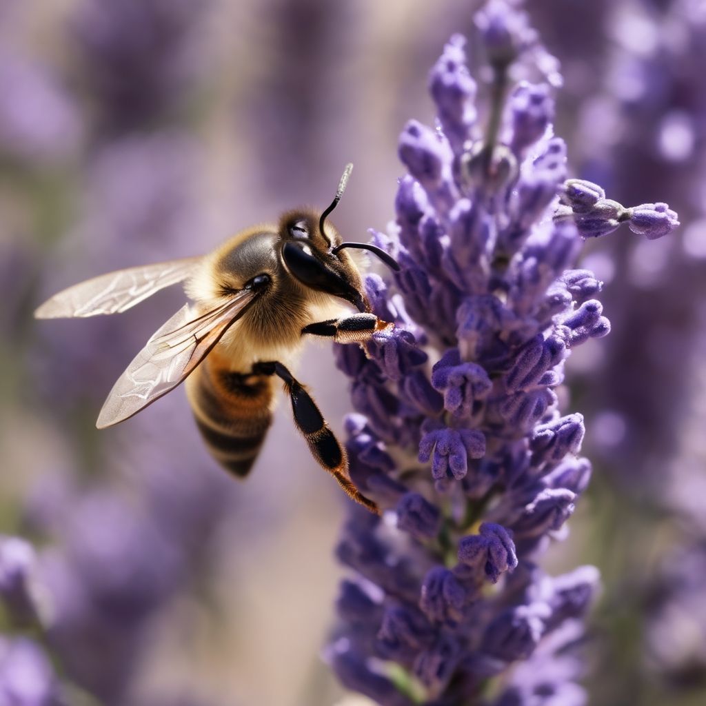


| Inference time | Memory | |
|---|---|---|
| Base | 14.1s | 11.24 GB |
| Stable Fast | 8.4s -40.43% | 12.11 GB +7.74% |
It more than meets expectations, you can see the great work behind this project.
The speed increase is one of the most notable in this article. The first image we generate takes a little longer (19s), but it's not important if we do warm up as in these tests.
The memory usage increases a bit but it's quite manageable.
As for the visual aspect, the composition changes slightly. In some images I would even say that the quality of certain elements has been increased, so.... seeing is believing.
When to use: I would say always.
DeepCache
DeepCache promises to be one of the best optimizations we can implement, with almost no drawbacks and easy to add. It makes use of a caching system to reuse high-level functions in addition to updating low-level functions in a more efficient way.
First we install the required library:
pip install deepcacheAnd then we integrate the following code into our pipeline:
- Python
from DeepCache import DeepCacheSDHelper

# ...

pipe = AutoPipelineForText2Image.from_pretrained(
  'stabilityai/stable-diffusion-xl-base-1.0',
  use_safetensors=True,
  torch_dtype=torch.float16,
  variant='fp16',
).to('cuda')

helper = DeepCacheSDHelper(pipe=pipe)
helper.set_params(cache_interval=3, cache_branch_id=0)
helper.enable()

generator = torch.Generator(device='cuda')

for i, generation in enumerate(queue, start=1):
  generator.manual_seed(generation['seed'])

  image = pipe(
    prompt=generation['prompt'],
    generator=generator,
  ).images[0]

  image.save(f'image_{i}.png')
There are two parameters that can be modified to achieve greater speed, although introducing greater loss of quality in the result.
cache_interval=3: Specifies how often the cache is updated in terms of steps.cache_branch_id=0: Specifies which branch of the neural network is responsible for executing the caching processes (in descending order,0is the first layer).
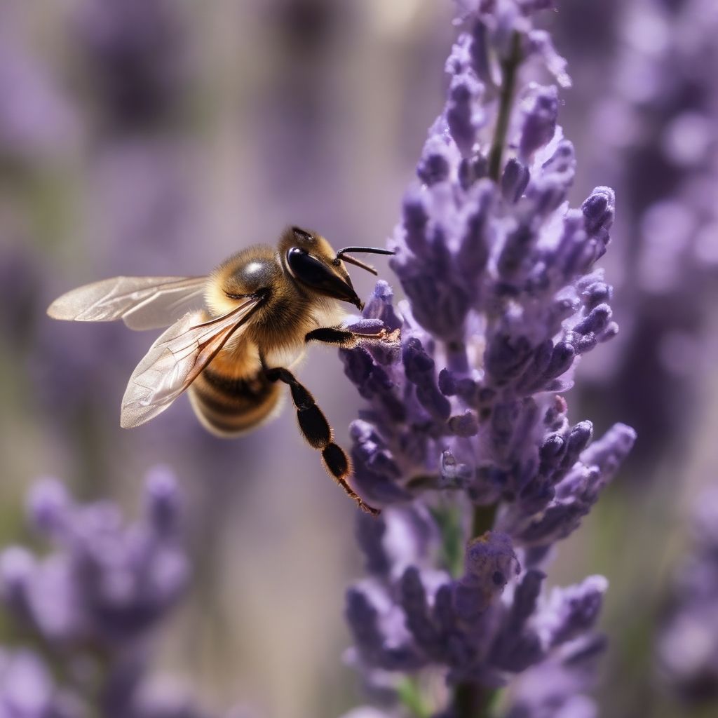
Let's see the result with the default recommended parameters.






| Inference time | Memory | |
|---|---|---|
| Base | 14.1s | 11.24 GB |
| DeepCache | 5.7s -59.57% | 11.58 GB +3.02% |
Wow. With a small penalty in memory usage, inference time can be reduced by more than half.
As for the image quality, you may have noticed that it changes quite a bit and, unfortunately, for the worse. Depending on the style of the image it may matter more or less, but the disadvantage is there (it doesn't seem to reduce the quality in images of objects very much).
Increasing the value of cache_branch_id seems to give a little more visual quality, although it may not be enough.
When to use: Since it reduces the inference time so much, it understandably reduces the quality of the result a bit. Without a doubt, to test prompts or parameters it's a very useful optimization. To use it in a process in which we seek a good result... I would say no.
TensorRT
TensorRT is a high-performance inference optimizer and runtime environment created by NVIDIA. It promises to accelerate the neural network inference process by breaking records.
But we already have a problem from the start. For the tests we're using pipelines from the diffusers library, and at the moment there is no pipeline compatible with TensorRT for Stable Diffusion XL. There are community pipelines for Stable Diffusion 2.x (txt2img, img2img or inpainting). I've also seen some stuff for Stable Diffusion 1.x, but as I said, not for SDXL.
On the other hand, in HuggingFace we can find the official stabilityai/stable-diffusion-xl-1.0-tensorrt repository. It contains instructions to perform the inference process with TensorRT, but unfortunately it uses quite complex scripts and practically impossible to adapt for these tests.
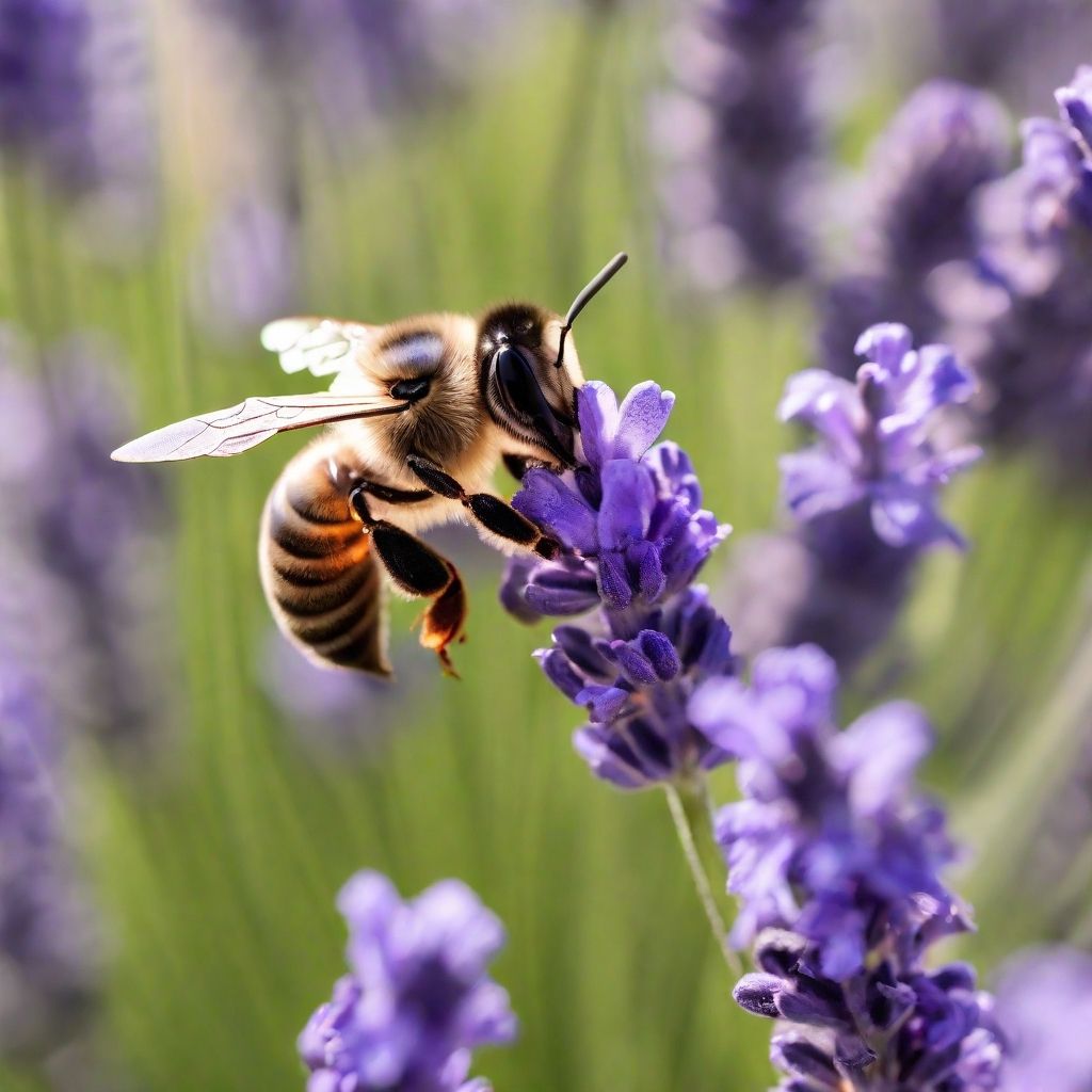
The results are going to look quite different because, to begin with, not even the same scheduler (Euler) is available in the scripts I've used. Still, I reused as many values as I could, including positive prompt, the absence of negative prompt, the same seed, the same CFG value, and the same image size.
I leave you the instructions to use this script in case you want to dig in:
# Clone the entire repository or download the files from this folder
# https://github.com/rajeevsrao/TensorRT/tree/release/8.6/demo/Diffusion

# Create and activate a virtual environment, as usual
python -m venv .venv

## Unix
source .venv/bin/activate
## Windows
.venv\Scripts\activate

# Install required libraries
pip install torch torchvision --index-url https://download.pytorch.org/whl/cu118
pip install transformers accelerate diffusers cuda-python nvtx onnx colored scipy polygraphy
pip install --pre --extra-index-url https://pypi.nvidia.com tensorrt
pip install --pre --extra-index-url https://pypi.ngc.nvidia.com onnx_graphsurgeon

# We can verify that TensorRT is installed correctly with the following line
python -c "import tensorrt; print(tensorrt.__version__)"
# 9.3.0.post12.dev1

# Perform inference
python demo_txt2img_xl.py "macro shot of a bee collecting nectar from lavender flowers"




| Compilation time | Inference time | |
|---|---|---|
| Base | 14.1s | |
| TensorRT | 34m | 8.2s -41.84% |
After preparing the models (something that takes about half an hour and only happens the first time), the inference process seems to speed up quite a lot, managing to generate each image in just 8 seconds, as opposed to 14 seconds for the non-optimized code. I can't talk about memory consumption because I would say that TensorRT uses different APIs.
About the quality of the images... they look amazing out of the box.
When to use: If you can integrate TensorRT in your process, go ahead. Seems like a good optimization and you should at least give it a try.
Component optimizations
These optimizations modify the various components of Stable Diffusion XL to improve its performance in several different ways. They may seem like small improvements but it all adds up.
torch.compile
Using PyTorch 2 or higher, we can compile models to obtain better performance thanks to the [torch.compile] API (https://pytorch.org/docs/stable/generated/torch.compile.html). While it's true that compilation takes time, successive calls will benefit from extra speed.
In previous versions of PyTorch, it was also possible to compile models with the tracing technique, through the torch.jit.trace API. This compilation at runtime (just-in-time / JIT) is less efficient than the new method, so we can forget about this API.
In the torch.compile method, the mode parameter accepts the following values: default, reduce-overhead, max-autotune and max-autotune-no-cudagraphs. In theory they're different but I haven't seen a difference, so we're going to use reduce-overhead.
If you use Windows you're in for a self-explanatory surprise:
RuntimeError: Windows not yet supported for torch.compile- Python
pipe = AutoPipelineForText2Image.from_pretrained(
  'stabilityai/stable-diffusion-xl-base-1.0',
  use_safetensors=True,
  torch_dtype=torch.float16,
  variant='fp16',
).to('cuda')

pipe.unet = torch.compile(pipe.unet, mode='reduce-overhead', fullgraph=True)

generator = torch.Generator(device='cuda')

for i, generation in enumerate(queue, start=1):
  generator.manual_seed(generation['seed'])

  image = pipe(
    prompt=generation['prompt'],
    generator=generator,
  ).images[0]

  image.save(f'image_{i}.png')
We're going to evaluate both the time it takes to compile the model and the time it takes for each successive generation.
| Compilation time | Inference time | Memory | |
|---|---|---|---|
| Base | 14.1s | 11.24 GB | |
torch.compile | 3m 34s | 12.5s -11.35% | 11.24 GB |
A simple optimization that quickly becomes profitable.
When to use: Whenever you're going to generate enough images to make it worth the compilation time.
OneDiff
OneDiff is an optimization library compatible with diffusers, ComfyUI and Stable Diffusion web UI from Automatic1111. The name literally means: one line of code to accelerate diffusion models.
It uses techniques such as quantization, improvements in attention mechanisms and compilation of models.
Installation is done by adding a couple of libraries, but if you are using another CUDA version or want to use a different installation method, check the documentation.
pip install --pre oneflow -f https://github.com/siliconflow/oneflow_releases/releases/expanded_assets/community_cu118

pip install --pre onediffIf you use Windows or macOS you will have to compile the library yourself.
RuntimeError: This package is a placeholder. Please install oneflow following the instructions in https://github.com/Oneflow-Inc/oneflow#install-oneflowThe creators also offer an Enterprise version that promises 20% extra speed (or even more), although I can't verify this and they don't give many details either.
Like torch.compile, the code required is a single line that alters the behavior of pipe.unet.
- Python
import oneflow as flow
from onediff.infer_compiler import oneflow_compile

# ...

pipe = AutoPipelineForText2Image.from_pretrained(
  'stabilityai/stable-diffusion-xl-base-1.0',
  use_safetensors=True,
  torch_dtype=torch.float16,
  variant='fp16',
).to('cuda')

pipe.unet = oneflow_compile(pipe.unet)

generator = torch.Generator(device='cuda')

with flow.autocast('cuda'):
  for i, generation in enumerate(queue, start=1):
    generator.manual_seed(generation['seed'])

    image = pipe(
      prompt=generation['prompt'],
      generator=generator,
    ).images[0]

    image.save(f'image_{i}.png')
Let's see if it lives up to expectations.


| Compilation time | Inference time | Memory | |
|---|---|---|---|
| Base | 14.1s | 11.24 GB | |
| OneDiff | 1m 25s | 7.8s -44.68% | 11.24 GB |
OneDiff introduces a slight change in the image structure, but it's a favorable change. In the interior image you can see how a bug is fixed by turning it into a shadow.
The compilation time is very low, much faster than torch.compile.
Regarding inference time, an impressive reduction of 45% is achieved, beating all competing optimizations (Stable Fast, TensorRT and torch.compile).
Surprisingly (and unlike Stable Fast), there is no increase in memory usage.
When to use: Always? It improves the visual quality of the result, almost halves inference time and the only penalty is a small wait at compilation time. What a great job!
Channels-last memory format
The channels-last memory format organizes the data so that the color channels are stored in the last dimension of the tensor.
By default the tensor has the NCHW format, which corresponds to the following four dimensions:
- N (Number): How many images to generate at the same time (batch size).
- C (Channels): How many channels the image has.
- H (Height): The height of the image in pixels.
- W (Width): The width of the image in pixels.
In contrast, with this technique the tensor data is reordered to be in NHWC format, putting the number of channels at the end.
- Python
pipe = AutoPipelineForText2Image.from_pretrained(
  'stabilityai/stable-diffusion-xl-base-1.0',
  use_safetensors=True,
  torch_dtype=torch.float16,
  variant='fp16',
).to('cuda')

pipe.unet.to(memory_format=torch.channels_last)

generator = torch.Generator(device='cuda')

for i, generation in enumerate(queue, start=1):
  generator.manual_seed(generation['seed'])

  image = pipe(
    prompt=generation['prompt'],
    generator=generator,
  ).images[0]

  image.save(f'image_{i}.png')
You can check if the tensor has been reordered with the following line (placing it before and after):
- Python
print(pipe.unet.conv_out.state_dict()['weight'].stride())Although it may improve efficiency in some cases and reduce memory usage, it's not compatible with some neural networks and could even worsen performance. Let's get rid of doubts!
| Inference time | Memory | |
|---|---|---|
| Base | 14.1s | 11.24 GB |
| Channels-last memory format | 14.1s | 11.24 GB |
The U-Net model in Stable Diffusion XL seems to not benefit from this optimization, but knowledge doesn't take up space, right?
When to use: Never, I guess.
FreeU
FreeU is the first and only optimization that does not improve inference time or memory usage, but the quality of the result.
This technique balances the contribution of two key elements in the U-Net architecture: skip connections (which introduce high-frequency details) and backbone feature maps (which provide semantics).
In other words, FreeU counteracts the introduction of unnatural details in the images, offering more realistic visual results.
- Python
pipe = AutoPipelineForText2Image.from_pretrained(
  'stabilityai/stable-diffusion-xl-base-1.0',
  use_safetensors=True,
  torch_dtype=torch.float16,
  variant='fp16',
).to('cuda')

pipe.enable_freeu(s1=0.9, s2=0.2, b1=1.3, b2=1.4)

generator = torch.Generator(device='cuda')

for i, generation in enumerate(queue, start=1):
  generator.manual_seed(generation['seed'])

  image = pipe(
    prompt=generation['prompt'],
    generator=generator,
  ).images[0]

  image.save(f'image_{i}.png')
You can play with these values although these are the recommended values for Stable Diffusion XL. More information in the project readme.




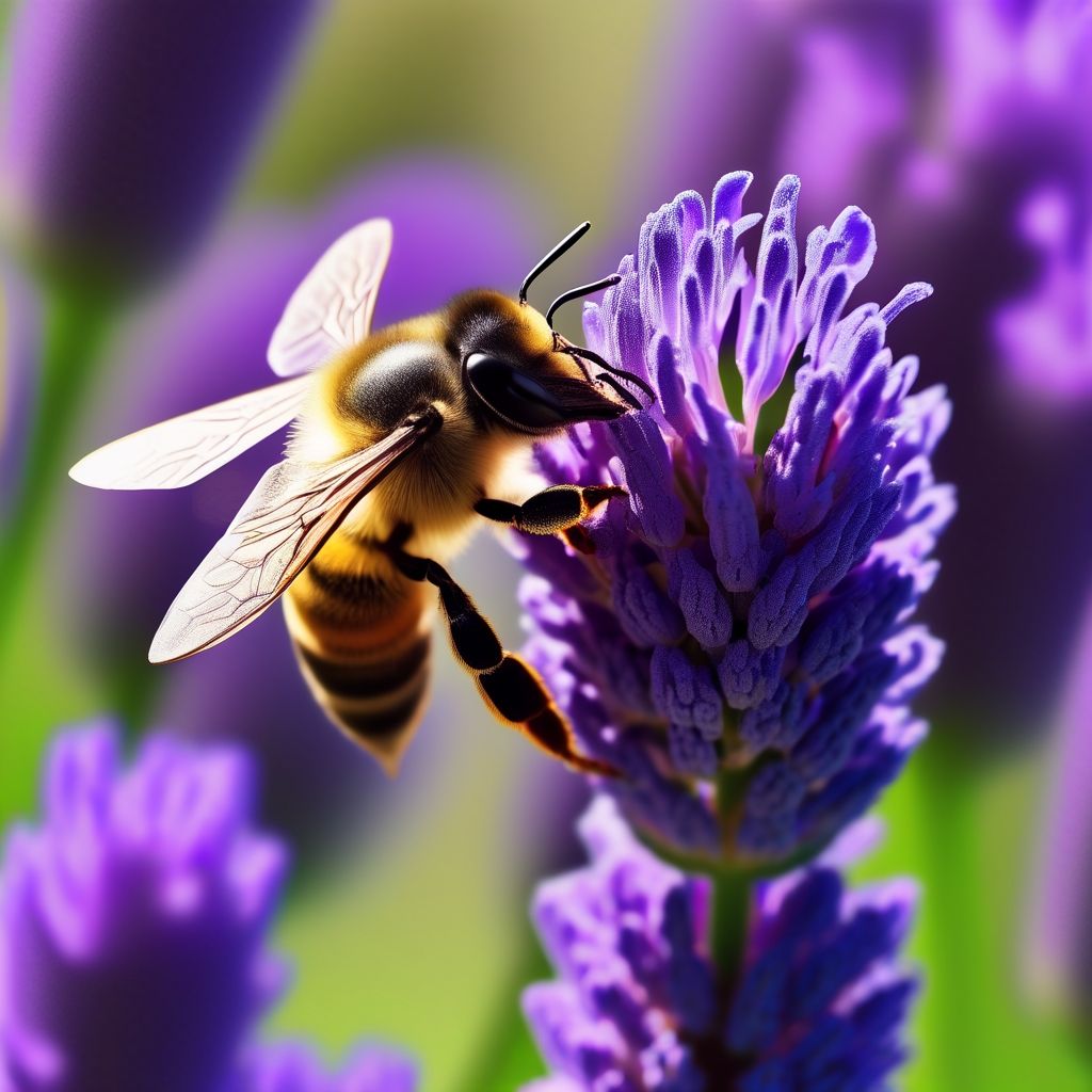


I had never tried FreeU before and the truth is that I didn't expect this result. I find images quite striking even though the structure is somewhat different from the original. It seems as if the image is more faithful to the prompt and focuses on delivering maximum visual quality instead of getting lost in small details.
The only negative point I see is that the image loses some coherence. For example, the sofa has a plant on top and the bee has 3 wings. I don't know, Rick...
When to use: When we want to achieve a more creative result with higher visual quality (although it also depends on the style we seek).
VAE FP16 fix
As we saw in the Batch processing optimization, the VAE included by default in Stable Diffusion XL does not work in FP16 format. Before decoding images, the pipeline executes a method that forces the model to work in FP32 format (pipe.upcast_vae()). And as we saw in the FP16 optimization, running a model in FP32 format is an unnecessary waste of resources.
The user madebyollin (also creator of TAESD, something we will see below) has created a patched version of this model so that it runs in FP16 format.
We just have to import this VAE and replace the original:
- Python
from diffusers import AutoPipelineForText2Image, AutoencoderKL

# ...

vae = AutoencoderKL.from_pretrained(
  'madebyollin/sdxl-vae-fp16-fix',
  use_safetensors=True,
  torch_dtype=torch.float16,
).to('cuda')

pipe = AutoPipelineForText2Image.from_pretrained(
  'stabilityai/stable-diffusion-xl-base-1.0',
  use_safetensors=True,
  torch_dtype=torch.float16,
  variant='fp16',
  vae=vae,
).to('cuda')

generator = torch.Generator(device='cuda')

for i, generation in enumerate(queue, start=1):
  generator.manual_seed(generation['seed'])

  image = pipe(
    prompt=generation['prompt'],
    generator=generator,
  ).images[0]

  image.save(f'image_{i}.png')


| Inference time | Memory | |
|---|---|---|
| Base | 14.1s | 11.24 GB |
| VAE FP16 | 13.9s -1.42% | 9.62 GB -14.41% |
There is no loss of quality, the images are practically the same.
In terms of memory usage we have managed to shave almost 15%, not bad at all for this simple change.
When to use: Always, unless you prefer to use the Tiny VAE optimization.
VAE slicing
When we generate several images at the same time (increasing the batch size), the VAE decodes all the tensors at the same time (in parallel). This considerably increases memory usage. To avoid this, the VAE slicing technique can be used to decode the tensors one by one (serially). Pretty much the same as we did manually in the Batch processing optimization.
Even if, for example, a batch size of 1, 2, 8 or 32 is used, the memory consumption by the VAE will remain the same, in exchange for a small time penalty that will be barely noticeable.
- Python
pipe = AutoPipelineForText2Image.from_pretrained(
  'stabilityai/stable-diffusion-xl-base-1.0',
  use_safetensors=True,
  torch_dtype=torch.float16,
  variant='fp16',
).to('cuda')

pipe.enable_vae_slicing()

generator = torch.Generator(device='cuda')

for i, generation in enumerate(queue, start=1):
  generator.manual_seed(generation['seed'])

  image = pipe(
    prompt=generation['prompt'],
    generator=generator,
  ).images[0]

  image.save(f'image_{i}.png')
When the batch size is 1 this optimization does nothing. And since we're using a batch size of 1 in these tests, we will skip the test results to see the veredict directly.
This optimization attempts to reduce memory usage when you increase batch size, which is precisely what increases memory usage the most. it's a contradiction in itself.
When to use: Only when you have a well-established process, so that you can generate several images at the same time and VAE execution is the bottleneck. That is, rarely.
VAE tiling
When we generate a high resolution image (4K / 8K), the VAE clearly becomes a bottleneck. Decoding an image of this size not only takes several minutes, but also uses an exorbitant amount of memory. it's not uncommon to end up getting the infamous error: torch.cuda.OutOfMemoryError: CUDA out of memory.
Through this optimization the tensor is split into several parts (as if they were tiles), then decoded one by one and finally rejoined again to form the image. This way the VAE does not have to decode everything at once.
- Python
pipe = AutoPipelineForText2Image.from_pretrained(
  'stabilityai/stable-diffusion-xl-base-1.0',
  use_safetensors=True,
  torch_dtype=torch.float16,
  variant='fp16',
).to('cuda')

pipe.enable_vae_tiling()

generator = torch.Generator(device='cuda')

for i, generation in enumerate(queue, start=1):
  generator.manual_seed(generation['seed'])

  image = pipe(
    prompt=generation['prompt'],
    generator=generator,
    height=4096,
    width=4096,
  ).images[0]

  image.save(f'image_{i}.png')
The areas where these parts have been joined may be noticeable due to some differences in color, but it's not common or easily perceived.
| Inference time | Memory | |
|---|---|---|
| Base | CUDA out of memory | |
| VAE tiling | 7m 51s | 12.45 GB |
This optimization is quite simple to understand: if you need to generate very high resolution images and your graphics card does not have enough memory, this will be the only option to achieve it.
When to use: Never. Very high resolution images contain flaws because Stable Diffusion has not been trained for this task. If you need to increase the resolution use an upscaler.
Tiny VAE
In the case of Stable Diffusion XL a 32-bit VAE with 50M parameters is used. Since this component is interchangeable we're going to use a VAE called TAESD. This small model with only 1M parameters is a distilled version of the original VAE that is also capable of running in 16 bit format.
- Python
from diffusers import AutoPipelineForText2Image, AutoencoderTiny

# ...

vae = AutoencoderTiny.from_pretrained(
  'madebyollin/taesdxl',
  use_safetensors=True,
  torch_dtype=torch.float16,
).to('cuda')

pipe = AutoPipelineForText2Image.from_pretrained(
  'stabilityai/stable-diffusion-xl-base-1.0',
  use_safetensors=True,
  torch_dtype=torch.float16,
  variant='fp16',
  vae=vae,
).to('cuda')

generator = torch.Generator(device='cuda')

for i, generation in enumerate(queue, start=1):
  generator.manual_seed(generation['seed'])

  image = pipe(
    prompt=generation['prompt'],
    generator=generator,
  ).images[0]

  image.save(f'image_{i}.png')
Is it worth sacrificing image quality for more speed and less memory usage? Let's take a look.




| Inference time | Memory | |
|---|---|---|
| Base | 14.1s | 11.24 GB |
| TAESD | 13.6s -3.55% | 7.57 GB -32.65% |
The reduction in memory usage is quite spectacular thanks to being a smaller model and capable of running in 16 bits.
The reduction in inference time is negligible.
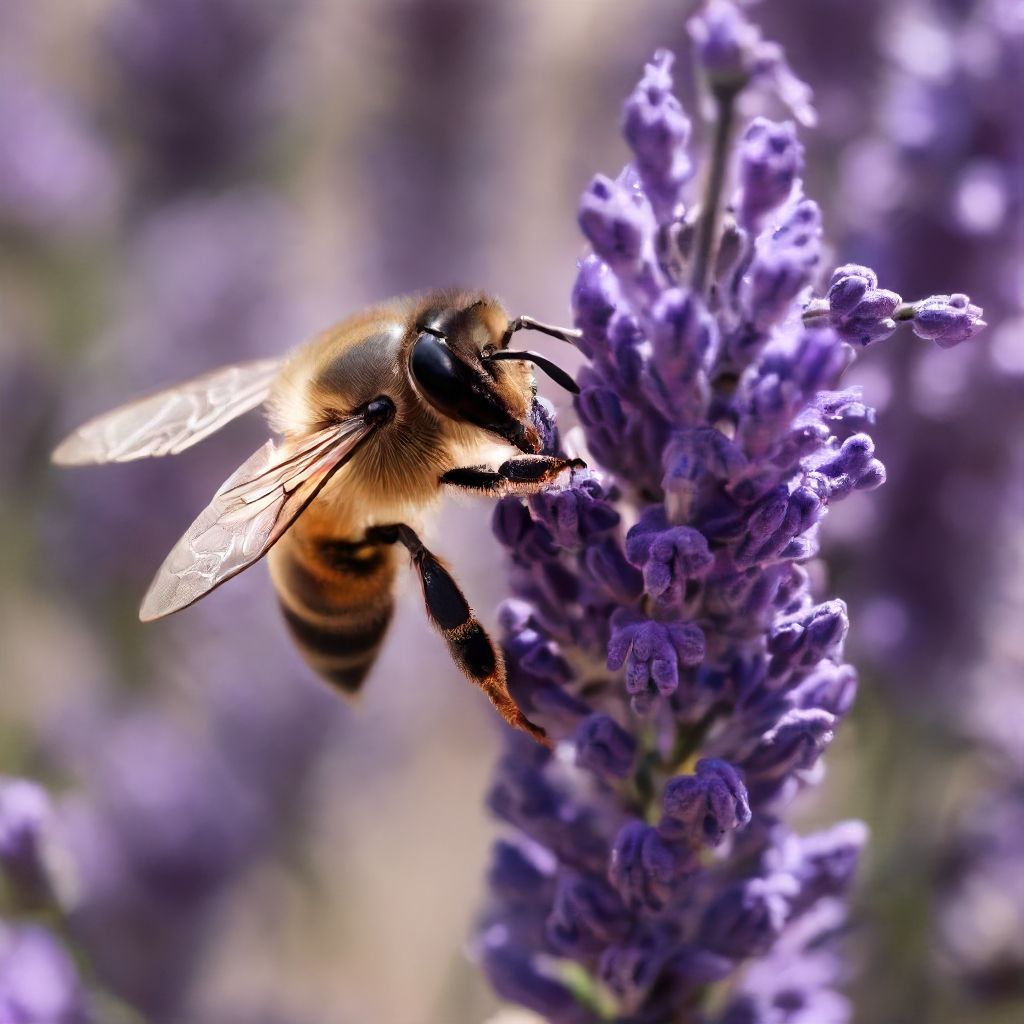
And what about the loss of quality? Well, as you can see, it's not noticeable. it's true that the image changes slightly, especially it seems to add a little more contrast and the textures a bit, but honestly I wouldn't be able to tell.
When to use: If you need to reduce memory usage, always. With this model and without using any other optimization, it's now possible to run the inference process on an 8 GB graphics card. If you're not forced to reduce memory usage, it would not be a bad idea to use it either because it does not seem to have a negative effect.
Parameter optimizations
In this category we will modify a couple of parameters to obtain extra speed in exchange for sacrificing image quality, with the expectation that it will not be noticeable.
Stable Diffusion XL uses Euler as the default sampler. Although there are some faster than others, Euler is in the category of fast samplers so changing it for another would not be considered an optimization.
Steps
By default SDXL uses 50 steps to clean a tensor full of noise. The more steps... more inference time, so there is room for improvement here. Using the num_inference_steps parameter, we can specify how many steps we want to use.
We're going to generate images with the following steps: 30, 25, 20 and 15. We will use the default value (50) as the basis for the comparison.
- Python
pipe = AutoPipelineForText2Image.from_pretrained(
  'stabilityai/stable-diffusion-xl-base-1.0',
  use_safetensors=True,
  torch_dtype=torch.float16,
  variant='fp16',
).to('cuda')

generator = torch.Generator(device='cuda')

for i, generation in enumerate(queue, start=1):
  generator.manual_seed(generation['seed'])

  image = pipe(
    prompt=generation['prompt'],
    num_inference_steps=30,
    generator=generator,
  ).images[0]

  image.save(f'image_{i}.png')
Of course... the fewer the steps, the shorter the inference time. What we're interested in is staying within the range of steps where quality and structure are maintained as much as possible. There is no point in saving a lot of time if we're going to obtain images worthy of the museum of horrors. Let's see where the limit is.









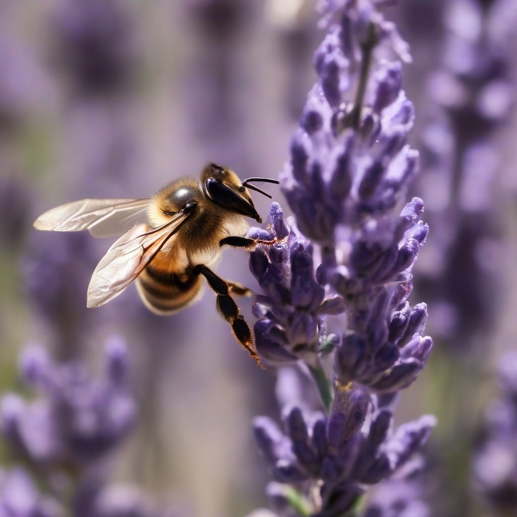
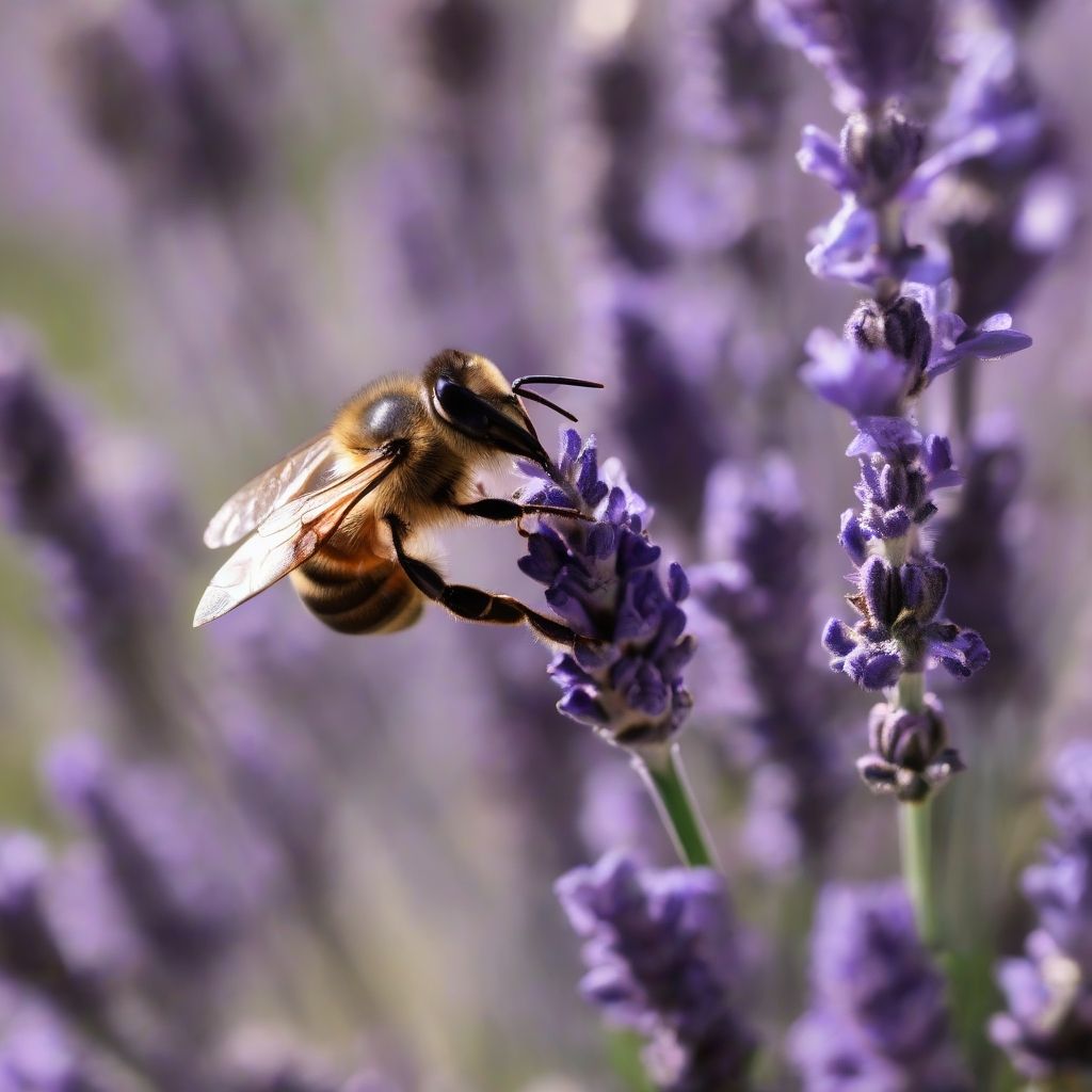
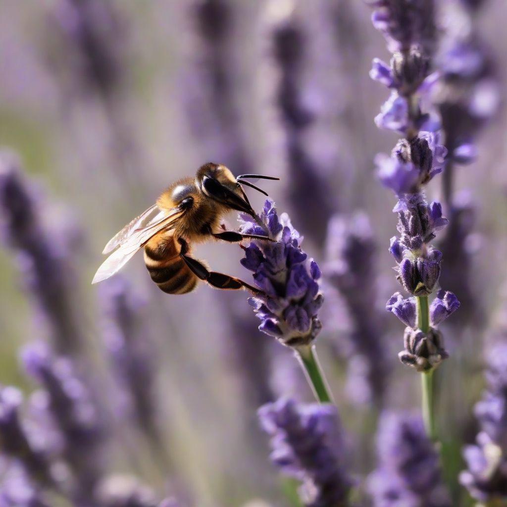


| Inference time | |
|---|---|
| Base (50 steps) | 14.1s |
| 40 steps | 11.2s -20.57% |
| 30 steps | 8.6s -39.01% |
| 25 steps | 7.3s -48.23% |
| 20 steps | 6.1s -56.74% |
| 15 steps | 4.8s -65.96% |
Portrait: At 15 and 20 steps the quality is not so bad, but the structure is different. At 25 steps and above I find the image quite correct.
Interior: At 15 steps you still don't get the desired structure. At 20 steps the result is quite decent as it's a creative image, but some elements are missing. So here too, I consider a minimum of 25 steps necessary. So here I also consider that at least 25 steps should be done.
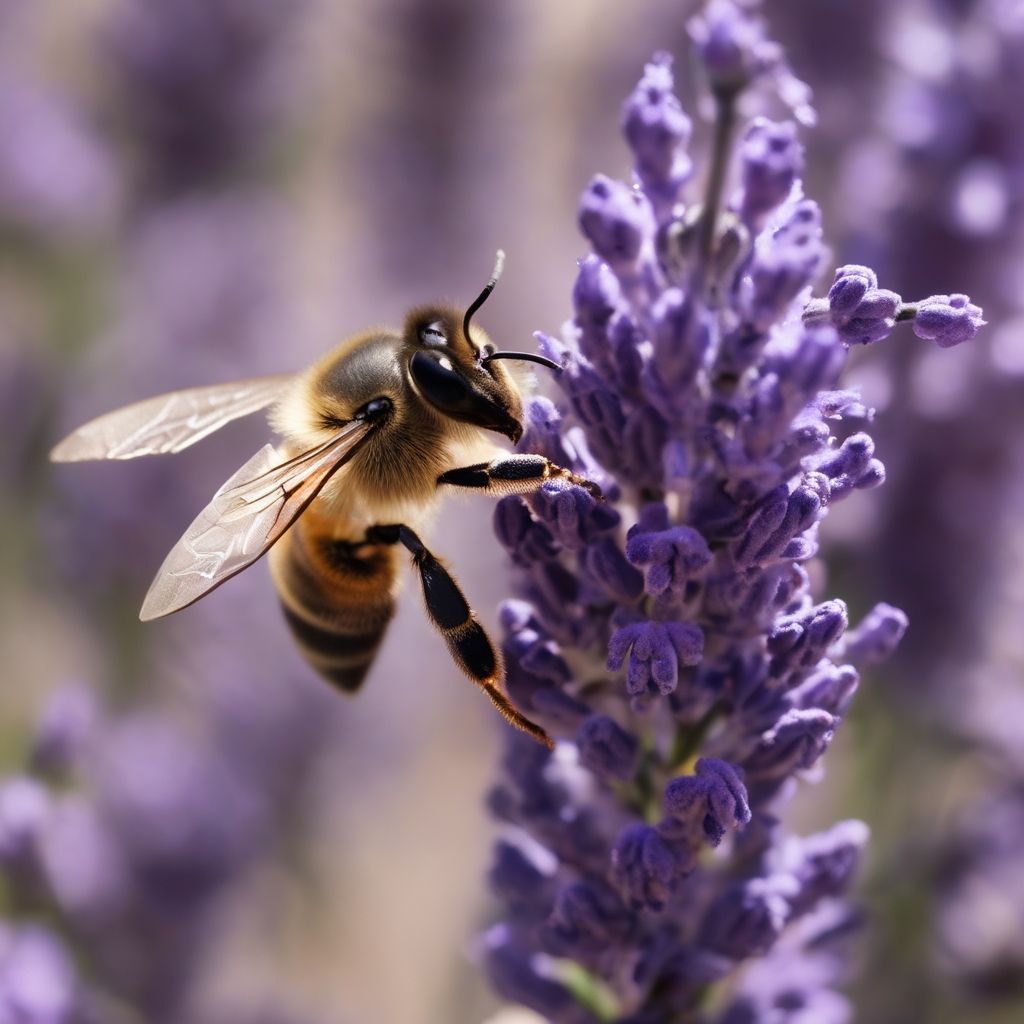
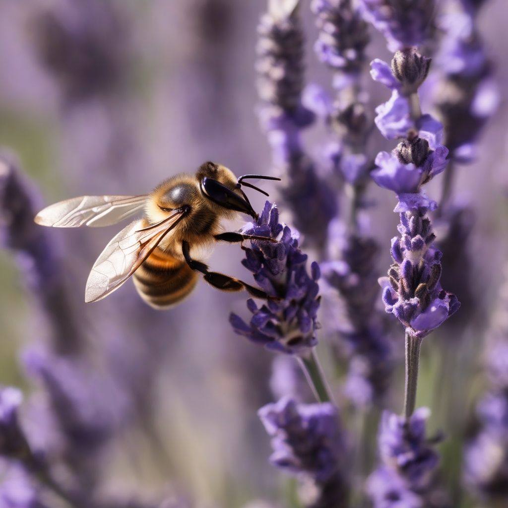
Macro: In macro photography the level of detail is amazing with just 15 steps. I wouldn't know which one to choose, they're all valid and correct.
3D: In a 3D-rendered style image there are too many defects with few steps, it even looks blurry in certain areas. Although the image in 30 steps is decent, here I would stay with the result after 50 steps (or maybe 40).
So, depending on the style of image you're generating you can use more or fewer steps, but in general you get quite good quality with 25-30 steps, which is a reduction in inference time of around 40%, which is a lot!
When to use: This is a great optimization when you're testing prompts or adjusting parameters and want to generate images quickly. When you have everything adjusted, you can go for maximum quality by increasing the number of steps. Depending on the use case it may even be permanent.
Disable CFG
As we saw in the article "How Stable Diffusion works", the classifier-free guidance (CFG) technique is responsible for bringing the noise predictor closer or further away from certain labels.
For example, if in the positive prompt we add the word car and in the negative prompt we add the word toy, the CFG value controls how close the noise predictor should get to the images associated with the termcar and how far it should move away from the territory where the images associated with the word toy are located. This is a very effective way to control the conditioning when generating images.
Then, in the article "How to implement Stable Diffusion", we saw how to implement the CFG technique and how it introduces the need to duplicate tensors:
- Python
# As we're using classifier-free guidance, we duplicate the tensor to avoid making two passes
# One pass will be for the conditioned values and another for the unconditioned values
latent_model_input = torch.cat([latents] * 2)
This means that the noise predictor takes twice as long to perform each step.
During the first steps, it's essential to have CFG active to obtain an image with good quality and faithful to our prompt. Once the noise predictor is on the right track, do we need to continue using CFG? In this optimization we're going to explore what happens when we stop using CFG during the process.
The code is simple, we create a function that is responsible for disabling CFG (pipe._guidance_scale = 0.0) when the number of steps has reached the value. Also, tensors will no longer be duplicated from this point on.
- Python
pipe = AutoPipelineForText2Image.from_pretrained(
  'stabilityai/stable-diffusion-xl-base-1.0',
  use_safetensors=True,
  torch_dtype=torch.float16,
  variant='fp16',
).to('cuda')

def callback_dynamic_cfg(pipe, step_index, timestep, callback_kwargs):
  if step_index == int(pipe.num_timesteps * 0.5):
    callback_kwargs['prompt_embeds'] = callback_kwargs['prompt_embeds'].chunk(2)[-1]
    callback_kwargs['add_text_embeds'] = callback_kwargs['add_text_embeds'].chunk(2)[-1]
    callback_kwargs['add_time_ids'] = callback_kwargs['add_time_ids'].chunk(2)[-1]
    pipe._guidance_scale = 0.0

  return callback_kwargs

generator = torch.Generator(device='cuda')

for i, generation in enumerate(queue, start=1):
  generator.manual_seed(generation['seed'])

  image = pipe(
    prompt=generation['prompt'],
    generator=generator,
    callback_on_step_end=callback_dynamic_cfg,
    callback_on_step_end_tensor_inputs=['prompt_embeds', 'add_text_embeds', 'add_time_ids'],
  ).images[0]

  image.save(f'image_{i}.png')
This function is executed at the end of each step as a callback, thanks to the callback_on_step_end parameter. We must also specify the tensors that we're going to modify inside the callback using the callback_on_step_end_tensor_inputs parameter.
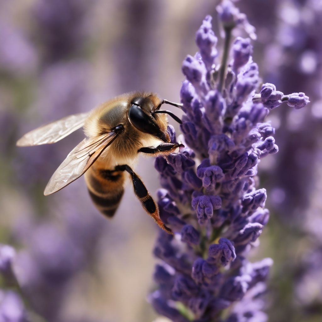
Let's explore what happens when we stop using CFG in the last quarter (75%) and in the second half of the process (50%).




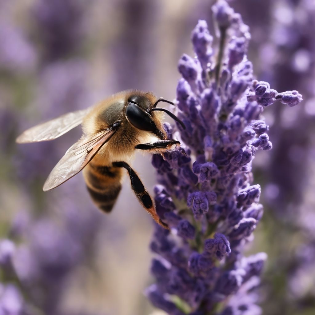


| Inference time | Memory | |
|---|---|---|
| Base | 14.1s | 11.24 GB |
| Disable CFG 75% | 12.6s -10.64% | 11.24 GB |
| Disable CFG 50% | 11.2s -20.57% | 11.24 GB |
As expected, deactivating CFG at 50% produces a 25% reduction in the inference time of each image (not the total, because model loading also counts). This is because if we perform 50 steps with CFG active, the model actually cleans 100 tensors. Instead, using this optimization, the model cleans 50 tensors in the first 25 steps and half (25 tensors) in the last 25 steps. So. 75/100 is equivalent to skipping 25% of the work. In the case of deactivating CFG at 75%, the reduction is 12.5% in each image.
As for the quality of the result, it seems to drop a bit but not too much. This may also be due to not having used a negative prompt, which is the main advantage of using CFG. Using better prompts is sure to increase the quality. At 75% it's practically imperceptible.
When to use: Aggressively, when you want to generate images faster and don't mind losing a bit of quality (for example, to test prompts or parameters). By deactivating CFG slightly later, speed increases without sacrificing quality.
Refiner
What about the refiner model? We have optimized the base model, but one of the main advantages of Stable Diffusion XL is that it has a specialized model that refines the small final details. This model significantly increases the quality of the result.
By default, the base model uses 11.24 GB of memory. When also using the refiner model, the memory requirements go up to 17.38 GB. But remember, most optimizations can also be applied to this model since it has the same components (except the first text encoder).
The warm up using the refiner model gets a bit complicated by having to warm up 2 different models. To do this, we get the result from the base model and pass it through the refiner model:
- Python
for generation in queue:
  image = base(generation['prompt'], output_type='latent').images
  refiner(generation['prompt'], image=image)
The refiner model can be used in two different ways, so let's look at them individually.
Ensemble of Expert Denoisers
The Ensemble of Expert Denoisers method refers to the approach in which image generation starts with the base model and ends with the refiner model. During the whole process no image is generated, but rather the base model cleans the tensor for a specified number of steps (a percentage of the total), and then passes the tensor to the refiner model to finish the job.
You could say that they work together to generate the result (base+refiner).
As for the code, the base model stops its work at 80% of the process using the denoising_end=0.8 parameter and returns the tensor thanks to output_type='latent'.
The refiner model receives this tensor via the image parameter (ironically, it's not an image). It then starts cleaning it assuming 80% of the work has already been done, indicated by the denoising_start=0.8 parameter. We also specify again how many steps the process has in total (num_inference_steps) so that it calculates how many steps it has left to clean. That is, if we use 50 steps with a change at 80%, the base model will clean the tensor for 40 steps and the refiner model for the last 10, refining the remaining details.
- Python
from diffusers import AutoPipelineForText2Image, AutoPipelineForImage2Image

# ...

base = AutoPipelineForText2Image.from_pretrained(
  'stabilityai/stable-diffusion-xl-base-1.0',
  use_safetensors=True,
  torch_dtype=torch.float16,
  variant='fp16',
).to('cuda')

refiner = AutoPipelineForImage2Image.from_pretrained(
  'stabilityai/stable-diffusion-xl-refiner-1.0',
  use_safetensors=True,
  torch_dtype=torch.float16,
  variant='fp16',
).to('cuda')

generator = torch.Generator(device='cuda')

for i, generation in enumerate(queue, start=1):
  generator.manual_seed(generation['seed'])

  image = base(
    prompt=generation['prompt'],
    generator=generator,
    num_inference_steps=50,
    denoising_end=0.8,
    output_type='latent',
  ).images # Remember that here we do not access images[0], but the entire tensor

  image = refiner(
    prompt=generation['prompt'],
    generator=generator,
    num_inference_steps=50,
    denoising_start=0.8,
    image=image,
  ).images[0]

  image.save(f'image_{i}.png')
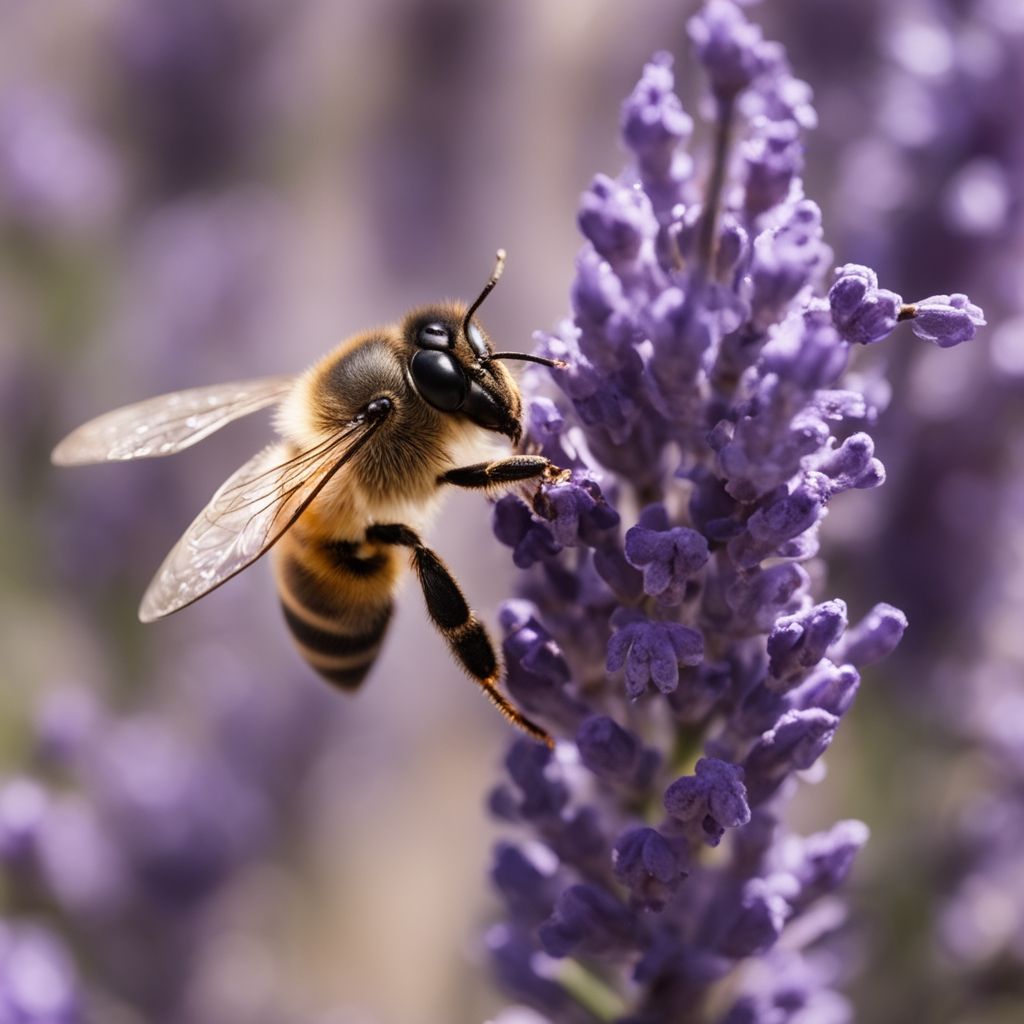
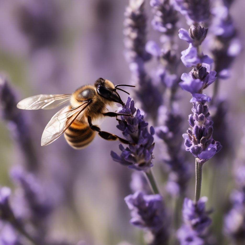
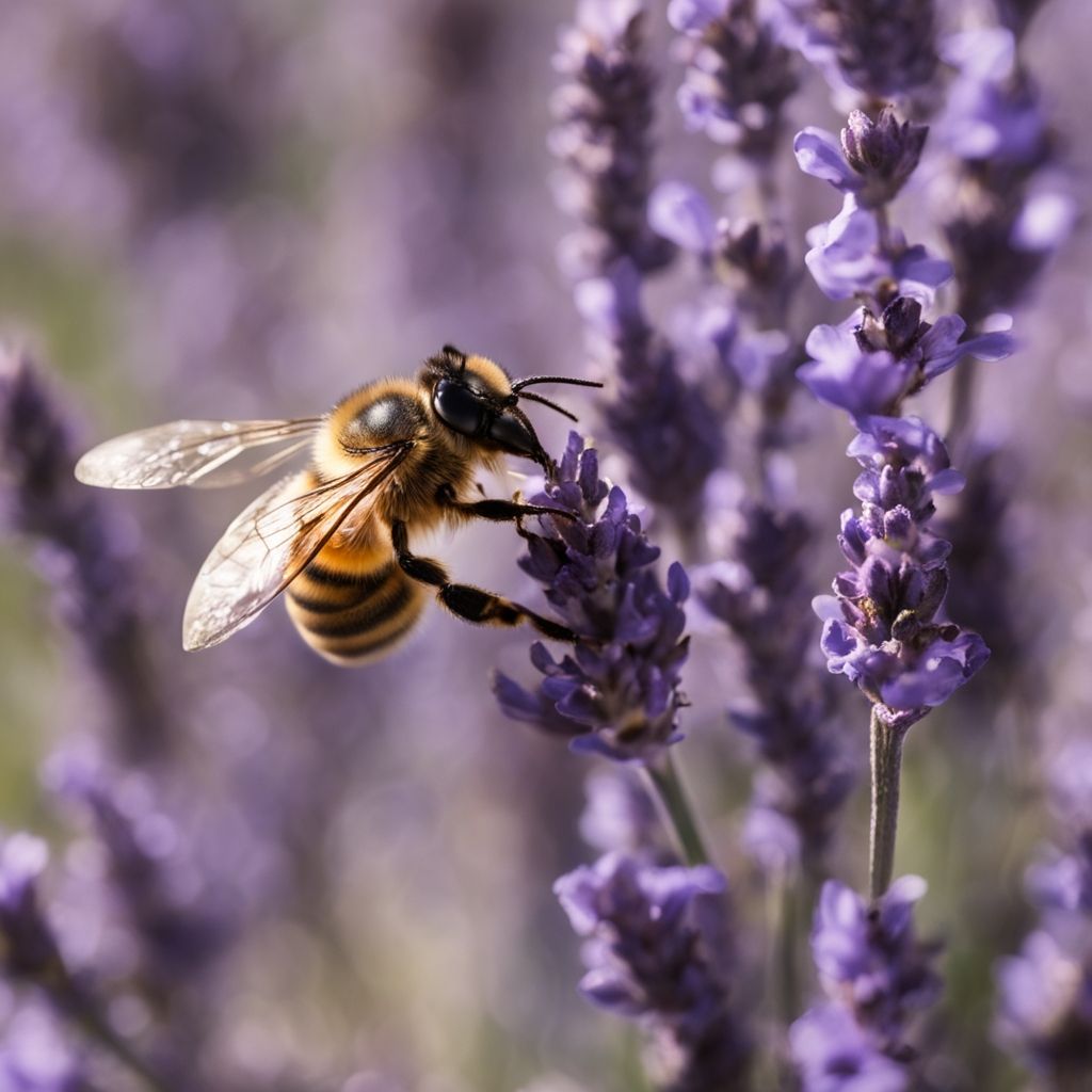
We're going to generate images in 50, 40, 30 and 20 steps, switching to the refiner model at 0.9 and 0.8.
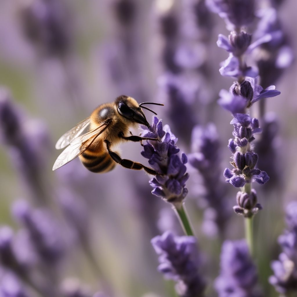
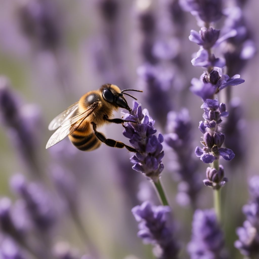
For reference, the image that has been used as the basis for all comparisons (base model only, 50 steps) will also be included.





| Inference time | |
|---|---|
| Base | 14.1s |
50 steps, 0.9 | 14.3s +1.42% |
50 steps, 0.8 | 14.5s +2.84% |
40 steps, 0.9 | 11.4s -19.15% |
40 steps, 0.8 | 11.5s -18.44% |
30 steps, 0.9 | 9s -36.17% |
30 steps, 0.8 | 9.1s -35.46% |
20 steps, 0.9 | 6.2s -56.03% |
20 steps, 0.8 | 6.3s -55.32% |
There is no doubt that using the refiner model greatly improves the result.
When is it better to take over? Clearly you can see how the results in 0.9 are better than in 0.8, which makes sense as it's a model that refines the final details and shouldn't be used to alter the image structure.
Regarding the number of steps, my perception is that the model is capable of delivering a result of very high visual quality regardless of the number of steps. The only thing that seems to change is the structure/composition of the image, but visual quality is high with only 30 steps.
And last but not least, we must also take into account the considerable reduction in time when going below 40 steps.
When to use: Whenever we want to use the refiner model to increase the visual quality of the image. As for the parameters, we could use 30 or 40 steps as long as we're not looking for the best possible quality. Of course, always making the change in 0.9.
Image-to-image
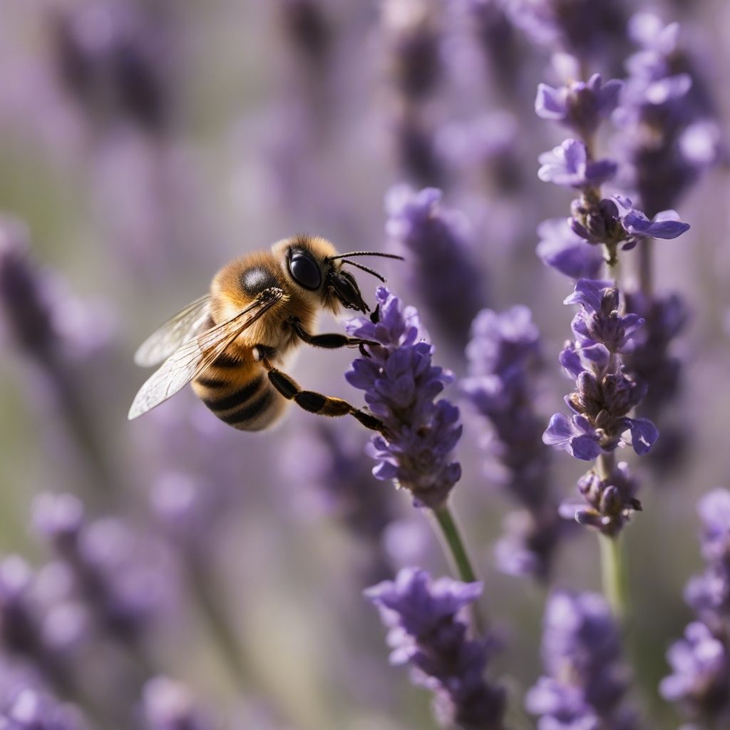
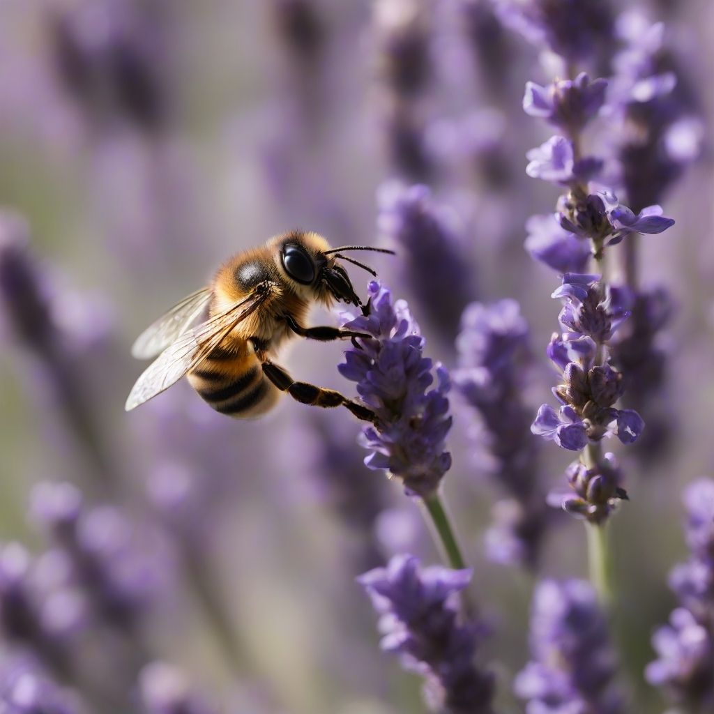
The classic img2img is nothing new in Stable Diffusion XL. This is the method in which a complete image is produced with the base model, and then both the image and the original prompt are passed to the refiner model, which generates a new image with these conditionings.
In other words, in img2img the models work independently (base->refiner).
Being two independent processes it's somewhat easier to apply the optimizations from this article. Nonetheless, the code is not very different, an image is simply generated and uses as a parameter in the refiner model.
- Python
from diffusers import AutoPipelineForText2Image, AutoPipelineForImage2Image

# ...

base = AutoPipelineForText2Image.from_pretrained(
  'stabilityai/stable-diffusion-xl-base-1.0',
  use_safetensors=True,
  torch_dtype=torch.float16,
  variant='fp16',
).to('cuda')

refiner = AutoPipelineForImage2Image.from_pretrained(
  'stabilityai/stable-diffusion-xl-refiner-1.0',
  use_safetensors=True,
  torch_dtype=torch.float16,
  variant='fp16',
).to('cuda')

generator = torch.Generator(device='cuda')

for i, generation in enumerate(queue, start=1):
  generator.manual_seed(generation['seed'])

  image = base(
    prompt=generation['prompt'],
    generator=generator,
    num_inference_steps=50,
  ).images[0]

  image = refiner(
    prompt=generation['prompt'],
    generator=generator,
    num_inference_steps=10,
    image=image,
  ).images[0]

  image.save(f'image_{i}.png')
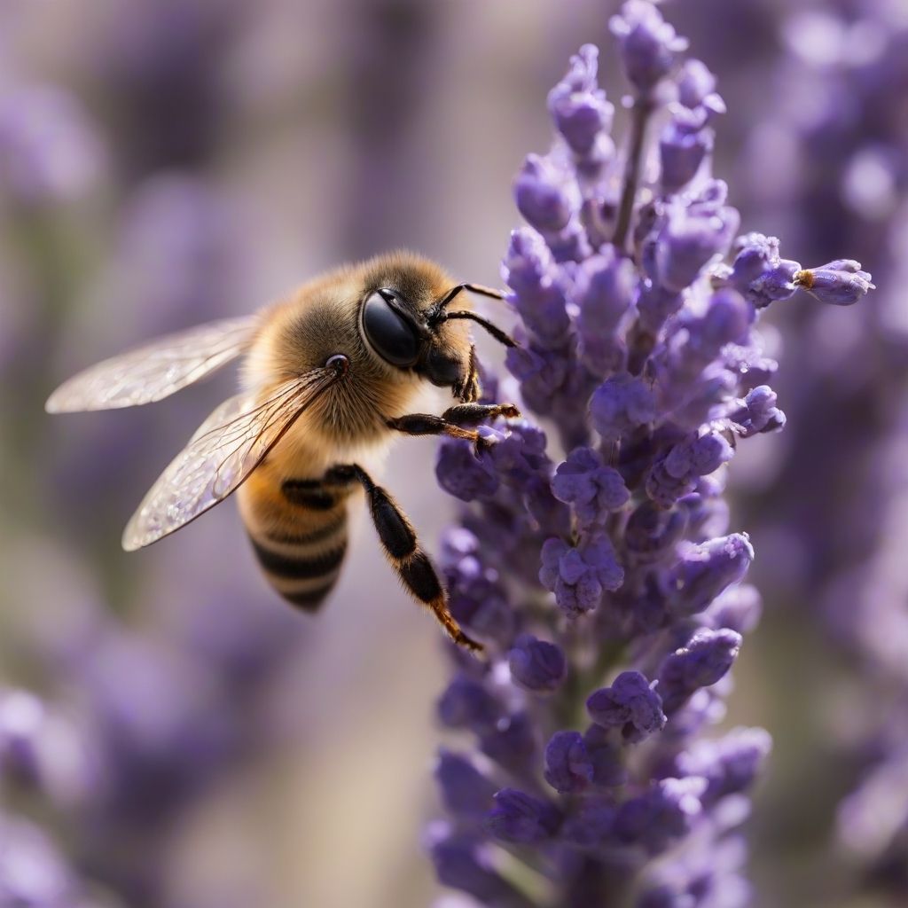
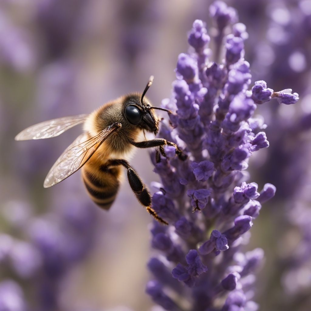
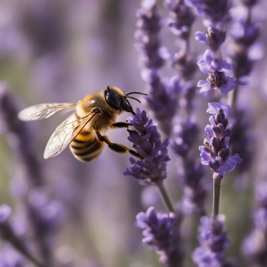
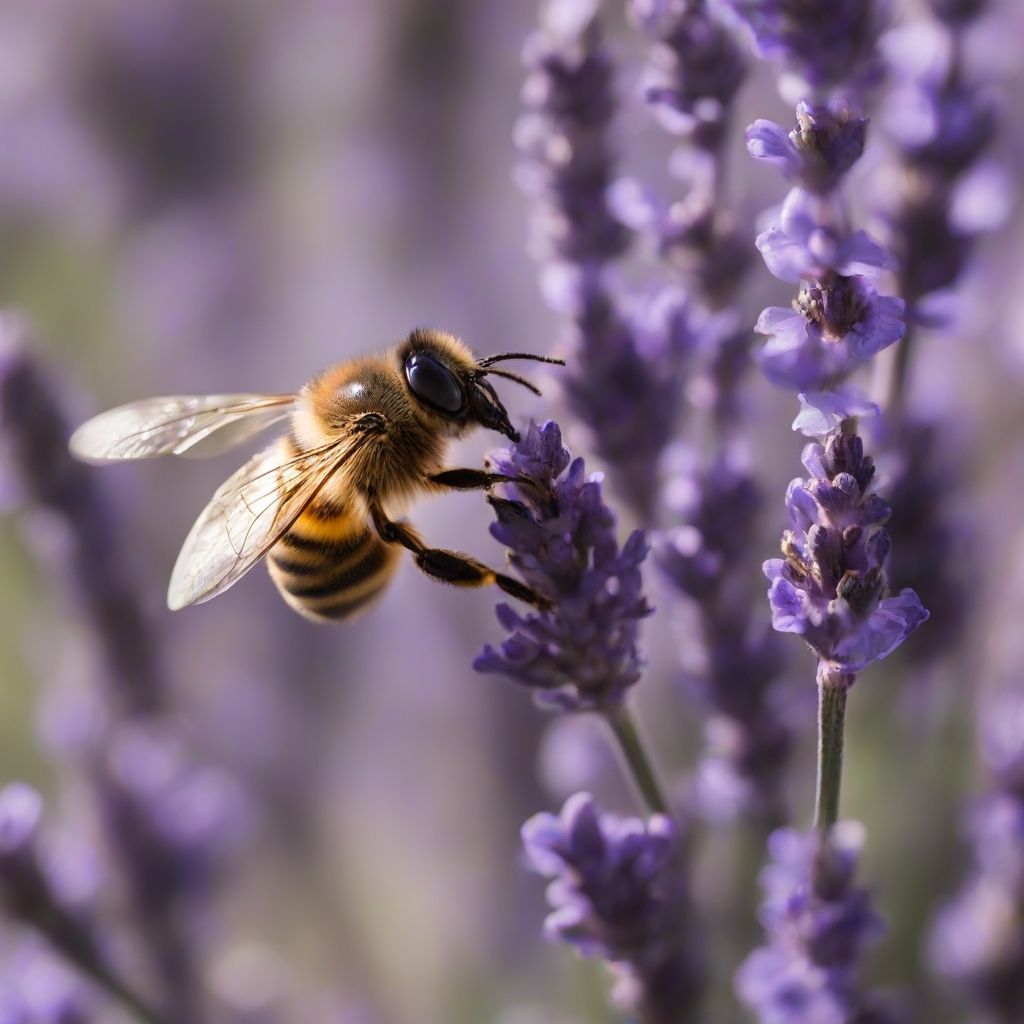
We're going to generate images with the base model at 50, 40, 30 and 20 steps, to then add a combination of 20 and 10 extra steps using the refiner model.
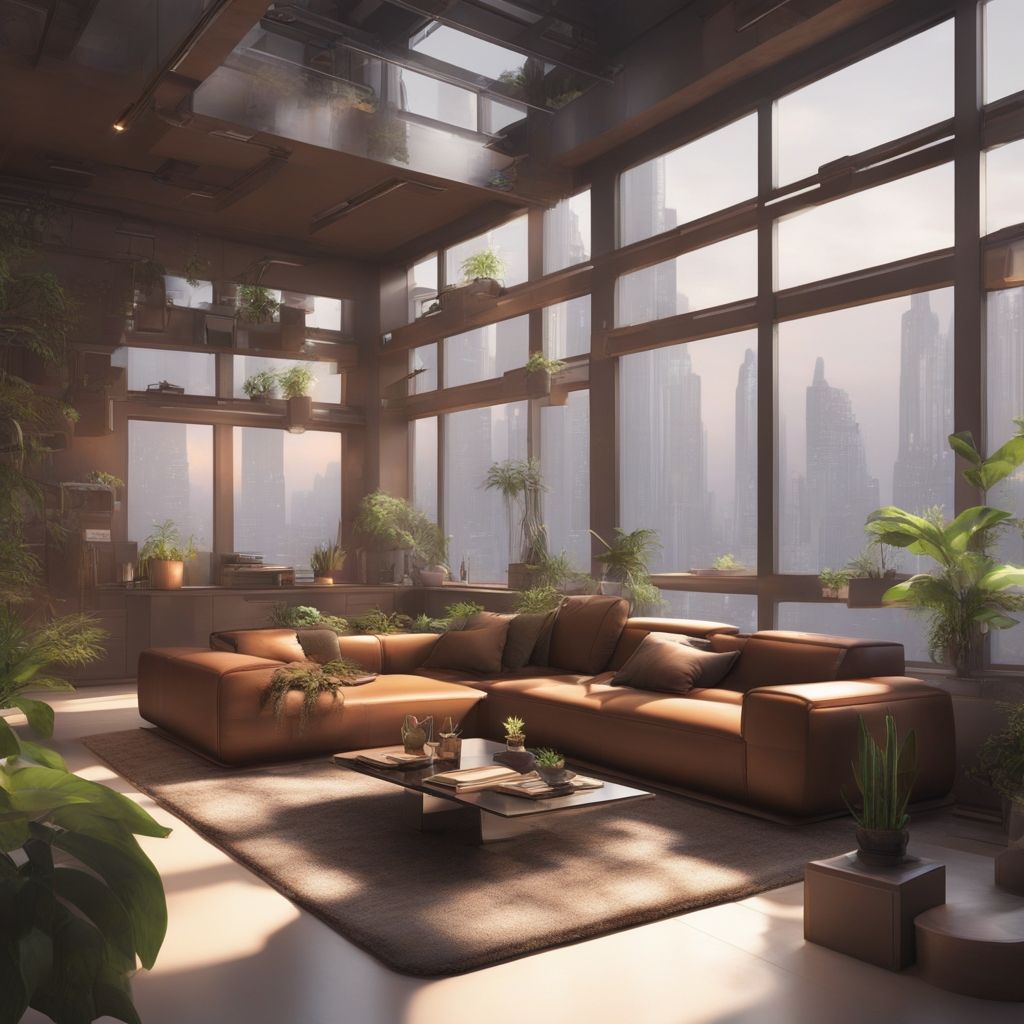
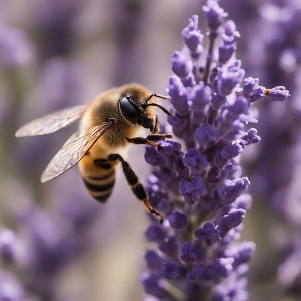
For reference, the image that has been used as the basis for all comparisons (base model only, 50 steps) will also be included.















| Inference time | |
|---|---|
| Base | 14.1s |
| 50 base + 20 refiner | 16.8s +19.15% |
| 50 base + 10 refiner | 15.6s +10.64% |
| 40 base + 20 refiner | 14.1s |
| 40 base + 10 refiner | 12.9s -8.51% |
| 30 base + 20 refiner | 11.5s -18.44% |
| 30 base + 10 refiner | 10.5s -25.53% |
| 20 base + 20 refiner | 8.9s -36.88% |
| 20 base + 10 refiner | 7.9s -43.97% |
In img2img mode the refiner model does not perform as well.
When we use enough steps with the base model, it looks like the refiner model is forced to add details to something that doesn't need it. As we say in our world: if something works, don't touch it.
On the other hand, if we use few steps in the base model the result is somewhat better. This happens because with so few steps, the base model isn't able to add the small details and gives some more room to work to the refiner model.
Here we also have to take into account the time reduction by decreasing the steps. If we use too many steps the penalty is significant.
When to use: The first thing to keep in mind is that when we use the refiner model is to maximize visual quality. In this use case it's convenient to increase the number of steps and therefore the Ensemble of Expert Denoisers method is the best option. With few steps I don't think there's better visual quality, nor does it increase generation speed compared to the other method. Therefore, using the refiner model in img2img mode falls into no man's land, it has its advantages but does not stand out in anything.
Conclusion
When I started this article I didn't think it would go this far. If you came here directly to see the conclusions, I don't blame you. However, if you've taken a look at all the optimizations I congratulate you and appreciate your perseverance (tap the emoji to celebrate). I hope you've learned from reading it as much as I did from writing it.
Depending on the objective and available hardware we will need to apply different optimizations. Let's summarize in a table all the optimizations and what kind of improvements (or penalties) they introduce.
The ones that appear as "neutral" are, in theory, a favorable change in that category but it's interpretable or only during some specific use case.
| Optimization | Alter result | Compilation | Quality | Time | Memory |
|---|---|---|---|---|---|
| CUDA and PyTorch versions | |||||
| Attention mechanisms | |||||
| FP16 | |||||
| TF32 | |||||
| Model CPU Offload | |||||
| Sequential CPU Offload | |||||
| Batch processing | |||||
| Stable Fast | |||||
| DeepCache | |||||
| TensorRT | |||||
| torch.compile | |||||
| OneDiff | |||||
| Channels-last memory format | |||||
| FreeU | |||||
| VAE FP16 fix | |||||
| VAE slicing | |||||
| VAE tiling | |||||
| Tiny VAE | |||||
| Steps | |||||
| Disable CFG | |||||
| Ensemble of Expert Denoisers | |||||
| Image-to-image |
If you value the effort I have put into this article and want to contribute so that I can dedicate more time to the blog and create new projects related to artificial intelligence, you can support me on Patreon or through Ko-fi. If you can afford it, thank you very much!
The shortest generation time with the base model with almost no quality loss, is achieved by using OneDiff + Tiny VAE + Disable CFG at 75% + 30 Steps.
With an RTX 3090 we can generate images in just 4.0s with a memory consumption of 6.91 GB, so it can even run on graphics cards with 8 GB of memory.
It is possible to add DeepCache to speed up the process even more. The problem is that it's not compatible with Disable CFG optimization and, by disabling it, the final speed ends up increasing.
Using this same configuration an A100 graphics card generates images in 2.7s. And with the brand new H100, the inference time is only 2.0s.
When using Sequential CPU Offload the bottleneck is in the VAE. Therefore, combining this optimization with VAE FP16 fix or Tiny VAE will result in a memory usage of 2.56 GB and 0.68 GB respectively. The memory usage is ridiculously low but the inference time will encourage you to get a new graphics card with more memory.
Using the Batch processing optimization decreases the memory usage to 5.77 GB, making it possible to generate images with Stable Diffusion XL on graphics cards with 6 GB of memory. There is no loss of quality or increase in generation time. And if we want to use the refiner model there is no problem, the memory consumption is the same.
Another option is to use Model CPU Offload which also reduces memory usage sufficiently, this time with a small time penalty.
With both techniques we can speed up the process a bit more by optimizing the VAE using VAE FP16 fix or Tiny VAE.
If we want to speed up the inference process a bit and generate images in 12.9s, we can achieve this by optimizing the VAE using VAE FP16 fix. And, if we don't mind altering the result a bit, we can further optimize by using Tiny VAE, lowering the memory consumption to 5.6 GB and the generation time to 12.6s.
And remember that other optimizations can still be applied to further reduce generation time.
Breaking the 6 GB barrier opens up new optimization options.
As we saw earlier, using OneDiff + Tiny VAE brings the memory usage down to 6.91 GB and achieves the lowest possible inference time. So if your graphics card has a minimum of 8 GB this is probably your best option.
You can support me so that I can dedicate even more time to writing articles and have resources to create new projects. Thank you!